Topic 3 Z-scores

Z-score are transformations of the data to create some standardization.

Here is how we calculate Z-scores:

$$\begin{equation} z=\frac{x_i-\overline{x}}{sd} \end{equation}$$

It is important to note that Z-scores always have:

• Mean = 0
• SD = 1

The shape of the Z-score distribution equals the shape of the distribution of the original values. We can check this with SPSS using the commands from Labs 1 and 2.

3.1 The Z-distribution

What if our original distribution was a normal distribution?

Because Z-scores standardize the values of any distribution, we can use them to generalize the properties of ANY normal distribution.

This idea is fundamental for inferential statistics.

The Z-distribution, therefore, is a distribution of Z-scores created from the values of a perfectly normal distribution.

3.2 Important concepts

3.2.1 Percentiles

Remember what percentile meant when you took the SATs or ACTs?

$95^{th}$ percentile = 750, means 95% of all values fall below 750.

Notation: The $X{th}$ percentile of a given variable is often referred to as $C_{X}$.

• E.g. $C_{95}$. is the $95{th}$ percentile of a given variable.

3.2.2 Quartiles

Equally divide the data into 4 percentiles: the $25^{th}$ percentile; the $50^{th}$ percentile; the $75^{th}$ percentile; the $100^{th}$ percentile.

Notation: There are only 4 quartiles. We define them as: $Q_{X}$.

• 1st quartile = $25^{th}$ percentile = $Q_{1}$
• 2nd quartile = $50^{th}$ percentile = $Q_{2}$
• 3rd quartile = $75^{th}$ percentile = $Q_{3}$
• 4th quartile = $100^{th}$ percentile = $Q_{4}$

Note: Since the 4th quartile is the highest value, we are often more concerned about $Q_{1}$, $Q_{2}$ and $Q_{3}$.

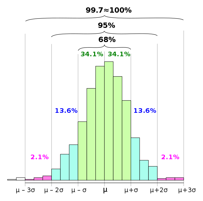
3.3 The empirical rules of the normal curve

Recall the rules of the normal curve from lecture (68%, 95% and 99%). Keep them in mind as we discuss Z-scores.

3.4 The Z-table

Because standard normal distributions are used very often, it is useful to have a table that summarizes its percentiles.

This is what Z-tables do. They give you the percentile for a given z value in a perfectly normal distribution. See the z-table at NYU classes.

3.5 Exercises

Part 1

Open the data set “Standard normal_N_10000.sav” from NYU classes.

This is a standard normal distribution with $n=10000$. We will use it to illustrate the properties of the standard normal and to understand the Z-table.

Using SPSS, perform the following commands:

1. Calculate measures of central tendency and measures of dispersion for the $x$ variable.
2. Check the histogram for the $x$ variable. Be sure to include a normal curve above it.
3. Create Z-scores for the values of $x$. SPSS will create the variable $Zx$.
4. Calculate measures of central tendency and measures of dispersion for the $Zx$ variable.
5. Check the histogram for the $Zx$ variable. Be sure to include a normal curve above it.
6. Calculate the 90th, 95th, 97.5th and 99th percentile of the $Zx$ distribution. Find those variables in the Z-table.

Part 2

Open the data set “earnings_data.sav” from NYU classes.

Perform the calculations in Part 1 for the variable $wages$.