11 Packages for Automated Exploratory Data Analysis
Below we showcase three packages DataExplorer, GGally, and skimr that have some nice EDA properties. While the thought of having an automated report is nice, what you find is that often you will still need to do quite a bit of cleaning to the data prior to getting all the output you want.
Wk4_Data <- 'C:/Users/jkyle/Documents/GitHub/Jeff_Data_Wrangling/Week_4/DATA'

library('kableExtra')
library('tidyverse')
#> -- Attaching packages --------------------------------------- tidyverse 1.3.1 --
#> v ggplot2 3.3.3     v purrr   0.3.4
#> v tibble  3.1.2     v dplyr   1.0.6
#> v tidyr   1.1.3     v stringr 1.4.0
#> v readr   1.4.0     v forcats 0.5.1
#> -- Conflicts ------------------------------------------ tidyverse_conflicts() --
#> x dplyr::filter()     masks stats::filter()
#> x dplyr::group_rows() masks kableExtra::group_rows()
#> x dplyr::lag()        masks stats::lag()

A_DATA_2 <- readRDS(file.path(Wk4_Data,'A_DATA_2.RDS'))

#A_DATA_TBL_2.t_ks_result.furrr <- readRDS(file.path(Wk4_Data,'A_DATA_TBL_2.t_ks_result.furrr.RDS'))

FEATURE_TYPE <- readRDS(file.path(Wk4_Data,'FEATURE_TYPE.RDS'))

numeric_features <- FEATURE_TYPE$numeric_features
categorical_features <- FEATURE_TYPE$categorical_features

sample_cat_features <- c('DIABETES', "Gender", "Race", "Marital_Status", "Pregnant", "yr_range", "Household_Icome")
sample_cont_features <- sample(numeric_features, 7, replace = FALSE )
For instance if we utilize the DataExplorer package on this week’s analysis data you will find it produces many bar graphs but the PCAs and Correlations will be missing from the report as the data has too many missing values.
11.1 DataExplorer
# SAMPLE R SCRPICT FOR DataExplorer create_report
library('tidyverse')

A_DATA <- readRDS('#TODO /Jeff_Data_Wrangling/Week_4/DATA/A_DATA.RDS')

colnames(A_DATA)

library('DataExplorer')

A_DATA %>%
  select(DIABETES, Age, Gender, Race, Birth_Country, Grade_Level, Marital_Status, Household_Icome, Poverty_Income_Ratio, BMXBMI, LBXGLU, PEASCTM1, BPXCHR) %>%
  mutate(DIABETES= as.factor(DIABETES)) %>%
    create_report(
        output_file  = "EDA_DataExplorer_DM2",
        output_dir   = "#TODO /Jeff_Data_Wrangling/Week_4",
        y            = "DIABETES",
        report_title = "EDA Report - NHANES Analysis Diabetes on A_DATA from Week 4"
    )
The DataExplorer create_report function will knit an EDA report HTML or other type of document to a file. There are many options
11.1.0.1 Reference
\(~\)
\(~\)
11.2 GGally
11.2.1 Categorigcal
GGally::ggpairs(A_DATA_2,
                columns = c(sample_cat_features),
                ggplot2::aes(color=as.factor(DIABETES)))
#> Registered S3 method overwritten by 'GGally':
#>   method from
#>   +.gg   ggplot2
#> `stat_bin()` using `bins = 30`. Pick better value with `binwidth`.
#> `stat_bin()` using `bins = 30`. Pick better value with `binwidth`.
#> `stat_bin()` using `bins = 30`. Pick better value with `binwidth`.
#> `stat_bin()` using `bins = 30`. Pick better value with `binwidth`.
#> `stat_bin()` using `bins = 30`. Pick better value with `binwidth`.
#> `stat_bin()` using `bins = 30`. Pick better value with `binwidth`.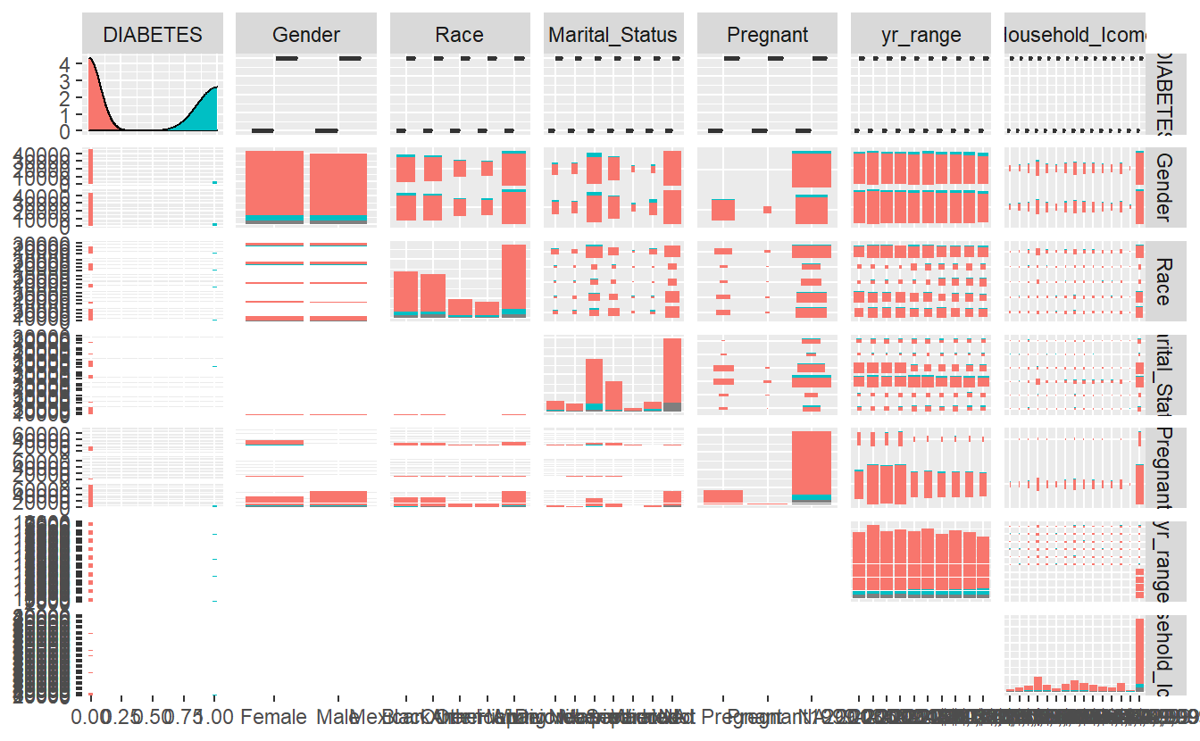
11.2.2 Continuous
GGally::ggpairs(A_DATA_2,
                columns = c(sample_cont_features),
                ggplot2::aes(color=as.factor(DIABETES)))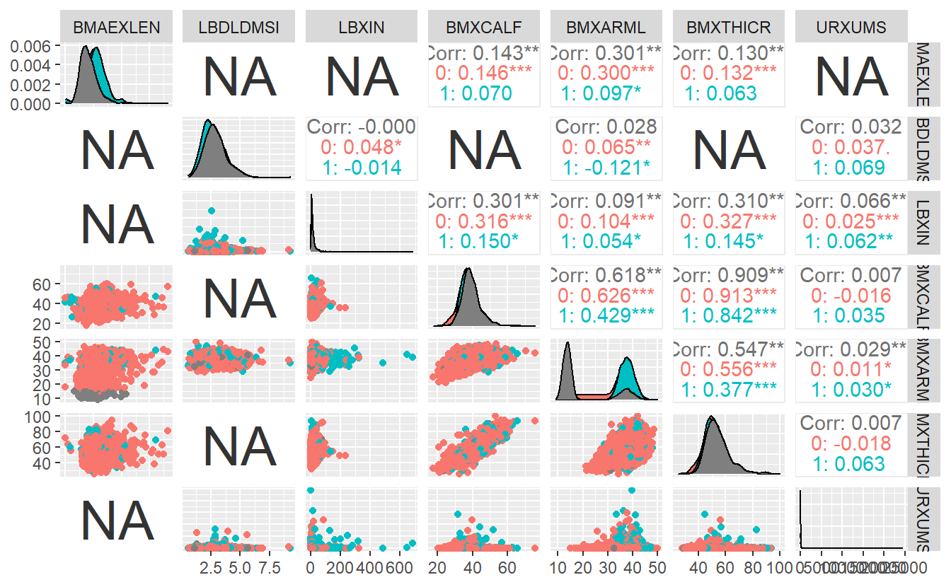
11.2.3 Mix and match
GGally::ggpairs(A_DATA_2,
                columns = c('DIABETES', "Gender", "Race", 'Age', 'BMIWT'),
                ggplot2::aes(color=as.factor(DIABETES)))
#> `stat_bin()` using `bins = 30`. Pick better value with `binwidth`.
#> `stat_bin()` using `bins = 30`. Pick better value with `binwidth`.
#> `stat_bin()` using `bins = 30`. Pick better value with `binwidth`.
#> `stat_bin()` using `bins = 30`. Pick better value with `binwidth`.
#> `stat_bin()` using `bins = 30`. Pick better value with `binwidth`.
#> `stat_bin()` using `bins = 30`. Pick better value with `binwidth`.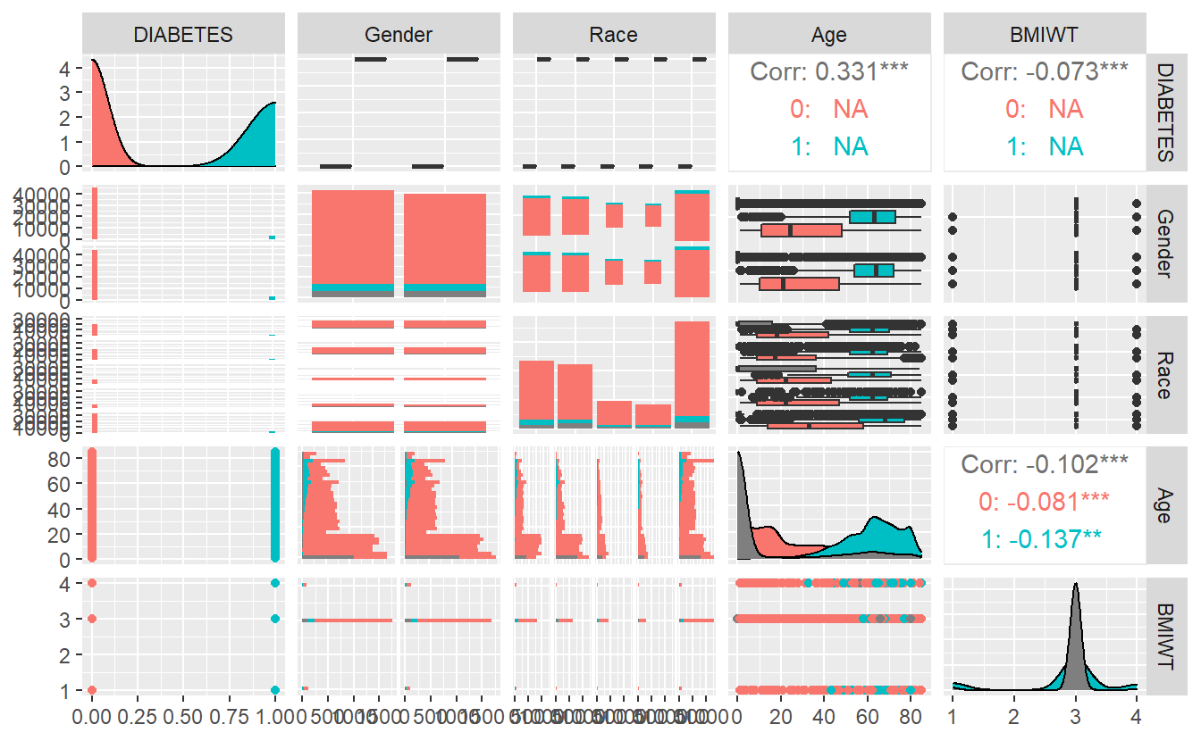
11.3 skimr
11.3.1 Reference
The output here is quite long so we will leave you with the reference first!
A_DATA_2 %>%
  select(c('DIABETES', all_of(sample_cont_features), all_of(sample_cat_features))) %>%
  group_by(DIABETES) %>%
skimr::skim()| Name | Piped data |
| Number of rows | 101316 |
| Number of columns | 14 |
| _______________________ | |
| Column type frequency: | |
| character | 6 |
| numeric | 7 |
| ________________________ | |
| Group variables | DIABETES |
Variable type: character
| skim_variable | DIABETES | n_missing | complete_rate | min | max | empty | n_unique | whitespace |
|---|---|---|---|---|---|---|---|---|
| Gender | 0 | 0 | 1.00 | 4 | 6 | 0 | 2 | 0 |
| Gender | 1 | 0 | 1.00 | 4 | 6 | 0 | 2 | 0 |
| Gender | NA | 0 | 1.00 | 4 | 6 | 0 | 2 | 0 |
| Race | 0 | 0 | 1.00 | 5 | 16 | 0 | 5 | 0 |
| Race | 1 | 0 | 1.00 | 5 | 16 | 0 | 5 | 0 |
| Race | NA | 0 | 1.00 | 5 | 16 | 0 | 5 | 0 |
| Marital_Status | 0 | 35025 | 0.61 | 7 | 19 | 0 | 6 | 0 |
| Marital_Status | 1 | 157 | 0.98 | 7 | 19 | 0 | 6 | 0 |
| Marital_Status | NA | 4620 | 0.20 | 7 | 19 | 0 | 6 | 0 |
| Pregnant | 0 | 71600 | 0.19 | 8 | 12 | 0 | 2 | 0 |
| Pregnant | 1 | 6219 | 0.09 | 8 | 12 | 0 | 2 | 0 |
| Pregnant | NA | 5611 | 0.03 | 8 | 12 | 0 | 2 | 0 |
| yr_range | 0 | 0 | 1.00 | 9 | 9 | 0 | 10 | 0 |
| yr_range | 1 | 0 | 1.00 | 9 | 9 | 0 | 10 | 0 |
| yr_range | NA | 0 | 1.00 | 9 | 9 | 0 | 10 | 0 |
| Household_Icome | 0 | 39949 | 0.55 | 13 | 18 | 0 | 14 | 0 |
| Household_Icome | 1 | 2422 | 0.64 | 13 | 18 | 0 | 14 | 0 |
| Household_Icome | NA | 2548 | 0.56 | 13 | 18 | 0 | 14 | 0 |
Variable type: numeric
| skim_variable | DIABETES | n_missing | complete_rate | mean | sd | p0 | p25 | p50 | p75 | p100 | hist |
|---|---|---|---|---|---|---|---|---|---|---|---|
| BMAEXLEN | 0 | 80419 | 0.09 | 263.65 | 79.13 | 0.00 | 214.00 | 260.00 | 307.00 | 909.00 | <U+2581><U+2587><U+2581><U+2581><U+2581> |
| BMAEXLEN | 1 | 6357 | 0.07 | 286.26 | 93.02 | 0.00 | 240.00 | 283.00 | 334.00 | 804.00 | <U+2581><U+2587><U+2583><U+2581><U+2581> |
| BMAEXLEN | NA | 5258 | 0.09 | 208.33 | 78.16 | 0.00 | 153.00 | 196.00 | 247.50 | 593.00 | <U+2581><U+2587><U+2583><U+2581><U+2581> |
| LBDLDMSI | 0 | 86573 | 0.02 | 2.82 | 0.91 | 0.62 | 2.17 | 2.74 | 3.36 | 9.15 | <U+2585><U+2587><U+2581><U+2581><U+2581> |
| LBDLDMSI | 1 | 6426 | 0.06 | 2.60 | 0.99 | 0.54 | 1.94 | 2.46 | 3.05 | 9.26 | <U+2587><U+2587><U+2581><U+2581><U+2581> |
| LBDLDMSI | NA | 5686 | 0.01 | 2.89 | 0.91 | 1.11 | 2.24 | 2.77 | 3.43 | 5.66 | <U+2583><U+2587><U+2585><U+2582><U+2581> |
| LBXIN | 0 | 70250 | 0.21 | 13.11 | 12.50 | 0.14 | 6.28 | 9.77 | 15.69 | 321.64 | <U+2587><U+2581><U+2581><U+2581><U+2581> |
| LBXIN | 1 | 4523 | 0.34 | 21.11 | 35.95 | 0.14 | 7.65 | 12.61 | 21.94 | 682.48 | <U+2587><U+2581><U+2581><U+2581><U+2581> |
| LBXIN | NA | 5335 | 0.08 | 16.68 | 13.12 | 2.28 | 8.44 | 12.59 | 20.71 | 84.65 | <U+2587><U+2582><U+2581><U+2581><U+2581> |
| BMXCALF | 0 | 60957 | 0.31 | 36.83 | 5.02 | 17.50 | 33.70 | 36.70 | 39.80 | 75.60 | <U+2581><U+2587><U+2582><U+2581><U+2581> |
| BMXCALF | 1 | 4996 | 0.27 | 38.21 | 4.79 | 24.30 | 34.90 | 37.70 | 41.00 | 65.70 | <U+2581><U+2587><U+2583><U+2581><U+2581> |
| BMXCALF | NA | 5468 | 0.05 | 39.06 | 4.97 | 24.20 | 35.90 | 38.60 | 41.60 | 59.00 | <U+2581><U+2587><U+2587><U+2582><U+2581> |
| BMXARML | 0 | 7633 | 0.91 | 33.46 | 6.72 | 11.50 | 31.00 | 35.50 | 38.00 | 49.90 | <U+2581><U+2582><U+2583><U+2587><U+2581> |
| BMXARML | 1 | 750 | 0.89 | 37.58 | 2.99 | 14.00 | 35.50 | 37.50 | 39.60 | 47.80 | <U+2581><U+2581><U+2581><U+2587><U+2581> |
| BMXARML | NA | 1122 | 0.81 | 19.46 | 10.34 | 9.00 | 13.00 | 14.30 | 17.50 | 47.00 | <U+2587><U+2581><U+2581><U+2582><U+2581> |
| BMXTHICR | 0 | 61284 | 0.31 | 51.25 | 8.01 | 25.10 | 46.20 | 50.70 | 55.90 | 100.00 | <U+2581><U+2587><U+2583><U+2581><U+2581> |
| BMXTHICR | 1 | 5065 | 0.26 | 52.44 | 7.87 | 29.20 | 47.00 | 51.50 | 56.80 | 93.90 | <U+2581><U+2587><U+2583><U+2581><U+2581> |
| BMXTHICR | NA | 5476 | 0.05 | 54.19 | 8.78 | 29.30 | 48.30 | 52.90 | 58.70 | 90.10 | <U+2581><U+2587><U+2585><U+2581><U+2581> |
| URXUMS | 0 | 38821 | 0.56 | 31.28 | 200.76 | 0.21 | 4.40 | 8.20 | 16.60 | 14800.00 | <U+2587><U+2581><U+2581><U+2581><U+2581> |
| URXUMS | 1 | 1967 | 0.71 | 172.30 | 793.23 | 0.30 | 6.50 | 15.60 | 52.82 | 24440.00 | <U+2587><U+2581><U+2581><U+2581><U+2581> |
| URXUMS | NA | 4809 | 0.17 | 50.26 | 231.67 | 0.21 | 4.80 | 10.00 | 21.30 | 4620.00 | <U+2587><U+2581><U+2581><U+2581><U+2581> |