3 Feature Engineering

Feature engineering is the process of transforming raw data into features that better represent the underlying measurements to be fed into the predictive model.

We will make use of our connection helper:

library('tidyverse')
#> -- Attaching packages --------------------------------------- tidyverse 1.3.1 --
#> v ggplot2 3.3.3     v purrr   0.3.4
#> v tibble  3.1.2     v dplyr   1.0.6
#> v tidyr   1.1.3     v stringr 1.4.0
#> v readr   1.4.0     v forcats 0.5.1
#> -- Conflicts ------------------------------------------ tidyverse_conflicts() --
#> x dplyr::filter() masks stats::filter()
#> x dplyr::lag()    masks stats::lag()

source('C:/Users/jkyle/Documents/GitHub/Jeff_Data_Wrangling/Functions/connect_help.R')
#> Warning: `src_sqlite()` was deprecated in dplyr 1.0.0.
#> Please use `tbl()` directly with a database connection

NHANES_Tables
#>  [1] "ACQ"      "ALB_CR"   "ALQ"      "ALQY"     "AUQ"      "BIOPRO"  
#>  [7] "BMX"      "BPQ"      "BPX"      "CBC"      "CDQ"      "CMV"     
#> [13] "COT"      "CRCO"     "DBQ"      "DEMO"     "DEQ"      "DIQ"     
#> [19] "DLQ"      "DPQ"      "DR1IFF"   "DR1TOT"   "DR2IFF"   "DR2TOT"  
#> [25] "DRXFCD"   "DS1IDS"   "DS1TOT"   "DS2TOT"   "DSBI"     "DSII"    
#> [31] "DSQIDS"   "DSQTOT"   "DUQ"      "DXX"      "DXXFEM"   "DXXSPN"  
#> [37] "Ds2IDS"   "ECQ"      "FASTQX"   "FERTIN"   "FETIB"    "FOLATE"  
#> [43] "FOLFMS"   "GHB"      "GLU"      "HDL"      "HEPA"     "HEPBD"   
#> [49] "HEPC"     "HEPE"     "HEQ"      "HIQ"      "HIV"      "HOQ"     
#> [55] "HSCRP"    "HSQ"      "HSV"      "HUQ"      "IHGEM"    "IMQ"     
#> [61] "INS"      "KIQ"      "LUX"      "MCQ"      "OCQ"      "OHQ"     
#> [67] "OHXDEN"   "OHXREF"   "OSQ"      "PAQ"      "PAQY"     "PBCD"    
#> [73] "PFAS"     "PFQ"      "PUQMEC"   "RHQ"      "RXQASA"   "RXQ_DRUG"
#> [79] "RXQ_RX"   "SLQ"      "SMQ"      "SMQFAM"   "SMQRTU"   "SMQSHS"  
#> [85] "SSPFAS"   "SXQ"      "TCHOL"    "TFR"      "TRIGLY"   "UCFLOW"  
#> [91] "UCM"      "UCPREG"   "UHG"      "UIO"      "UNI"      "VIC"     
#> [97] "VOCWB"    "VTQ"

\(~\)

3.1 Features and Targets

Definition 3.1 A feature is an individual measurable property or characteristic of a phenomenon being observed that can be used for analysis; some examples might include patient attributes such as Height, Weight, Age, or Gender. Depending on the prediction task or analysis, the features you include in the analytic data-set can widely vary. Features might also be thought-of or called:

independent variables
predictor variables
input variables
covariates
explanatory variables
risk factors

depending on the context.

\(~\)

Definition 3.2 A target is a feature of interest we wish to gain a deeper understanding, analyze, or make a predictions on. Also called response or label, we often think of these as the dependent variable or outcome.

Targets in medical machine learning models typically include adverse events or clinical outcomes to various treaments or cohort designed studies.

\(~\)

Definition 3.3 Data leakage is when information that would not normally be available to the model leaks into the training data-set.

\(~\)

For the majority of these exercises we will examine the process of data science with our primary example, we will consider Diabetes from the NHANES database as our primary outcome, all other available data with-in the data-base should be examined for it’s potential to be transformed into features.

3.2 Example : Diabetes

The target will be a “Yes” response to the question DIQ010:

The next questions are about specific medical conditions. {Other than during pregnancy, {have you/has SP}/{Have you/Has SP}} ever been told by a doctor or health professional that {you have/{he/she/SP} has} diabetes or sugar diabetes?

Identification of the features for models is often an iterative and ongoing process.

Example 3.1 Hypothetically speaking, any respondent that has diabetes, has a date at which they first learned that they had diabetes.

Another expectation we might have is that: every respondent that reported a valid age at which they first learned of diabetes, also probably respondeded “Yes” to question DIQ010

Within the context of predicting Diabetes: if we already know the respondent’s age at which they first learned they had diabetes, then we expect the patient already has diabetes; this would be a good example of data leakage.

3.3 Features and Targets Vary by Prediction Task.

If we instead chose a prediction task on “depression.” Then our features, targets, and potential data-leakages all change.

3.3.1 Example : Depression

Open_NHANES_table_help('DPQ')

The target might be derived from one of the following:

DPQ010 - “Have little interest in doing things”
DPQ020 - “Feeling down, depressed, or hopeless”
DPQ060 - “Feeling bad about yourself”
DPQ090 - “Thought you would be better off dead”
DPQ100 - “Difficulty these problems have caused”

Notice now, in this context, Age at Diabetes is no longer leaking into the relationship with the target of Depression.

\(~\)

3.4 Define Targets - Diabetes and Age at Diabetes

Back to our primary example we will consider the task of modeling Diabetics.

DIQ <- tbl(NHANES_DB, "DIQ")

Open_NHANES_table_help('DIQ')

3.5 Diabetes

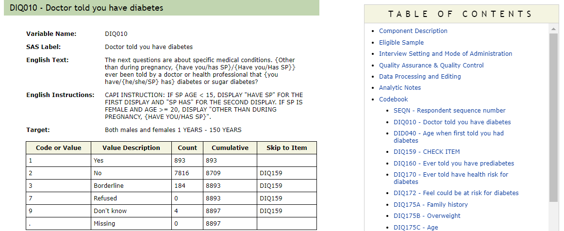
We will use the DIQ010 column to identify members who have DIABETES :


DM2_TBL <- DIQ %>%
  mutate(DIABETES = 
           case_when(DIQ010 == 1 ~ 1,
                     DIQ010 == 2 ~ 0,
                     (DIQ010 !=1 | DIQ010 !=2) ~ NA)
         ) %>%
  select(SEQN, DIABETES)

DM2_TBL %>%
  glimpse()
#> Rows: ??
#> Columns: 2
#> Database: sqlite 3.35.5 [C:\Users\jkyle\Documents\GitHub\Jeff_Data_Mgt_R_PRV\DATA\sql_db\NHANES_DB.db]
#> $ SEQN     <dbl> 1, 2, 3, 4, 5, 6, 7, 8, 9, 10, 11, 12, 13, 14, 15, 16, 17, 18~
#> $ DIABETES <dbl> 0, 0, 0, 0, 0, 0, 0, 0, 0, 0, 0, 0, 1, 0, 0, 0, 0, 0, 0, 0, 0~

3.6 Age at Diabetes

Some features will be easier to define than others, as we shall see here. Above it was relatively easy to create a flag for DIABETES. However if we consider a similar but related data-point the Age at which the member first learned of their diagnosis it is more complicated:

3.6.1 Analytic Notes on DIQ

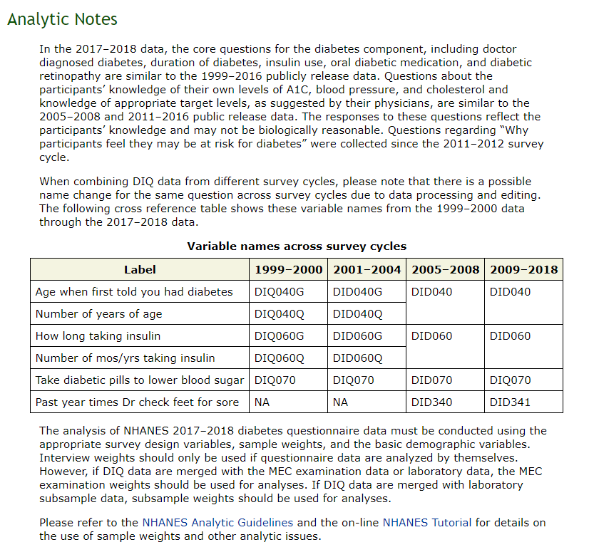
As per the Analytic notes on the DIQ table the “Age at Diabetes” has been mapped to different source variables over the number of years that the survey has been deployed. From the notes it appears that AGE_AT_DIAG_DM2 is recorded across DIQ040G, DIQ040Q, DID040G, DID040Q, DID040 depending on the yr_range.

We might want to review each of the ranges in the above table to check our understanding of the data:

3.6.2 DIQ : Age at Diabetes : 1991-2000

DIQ %>%
  select(SEQN, yr_range, DIQ040G, DIQ040Q, DID040G, DID040Q, DID040) %>%
  filter('1991-2000') %>%
  filter(!is.na(DIQ040G)) %>%
  glimpse()
#> Rows: ??
#> Columns: 7
#> Database: sqlite 3.35.5 [C:\Users\jkyle\Documents\GitHub\Jeff_Data_Mgt_R_PRV\DATA\sql_db\NHANES_DB.db]
#> $ SEQN     <dbl> 13, 29, 40, 55, 71, 83, 130, 148, 163, 187, 266, 272, 274, 30~
#> $ yr_range <chr> "1999-2000", "1999-2000", "1999-2000", "1999-2000", "1999-200~
#> $ DIQ040G  <dbl> 1, 1, 1, 1, 1, 1, 1, 1, 1, 1, 1, 1, 1, 1, 1, 1, 1, 1, 2, 1, 1~
#> $ DIQ040Q  <dbl> 67, 61, 63, 57, 60, 57, 1, 76, 56, 66, 20, 19, 32, 60, 99999,~
#> $ DID040G  <dbl> NA, NA, NA, NA, NA, NA, NA, NA, NA, NA, NA, NA, NA, NA, NA, N~
#> $ DID040Q  <dbl> NA, NA, NA, NA, NA, NA, NA, NA, NA, NA, NA, NA, NA, NA, NA, N~
#> $ DID040   <dbl> NA, NA, NA, NA, NA, NA, NA, NA, NA, NA, NA, NA, NA, NA, NA, N~

Open_NHANES_table_help('DIQ','1999-2000')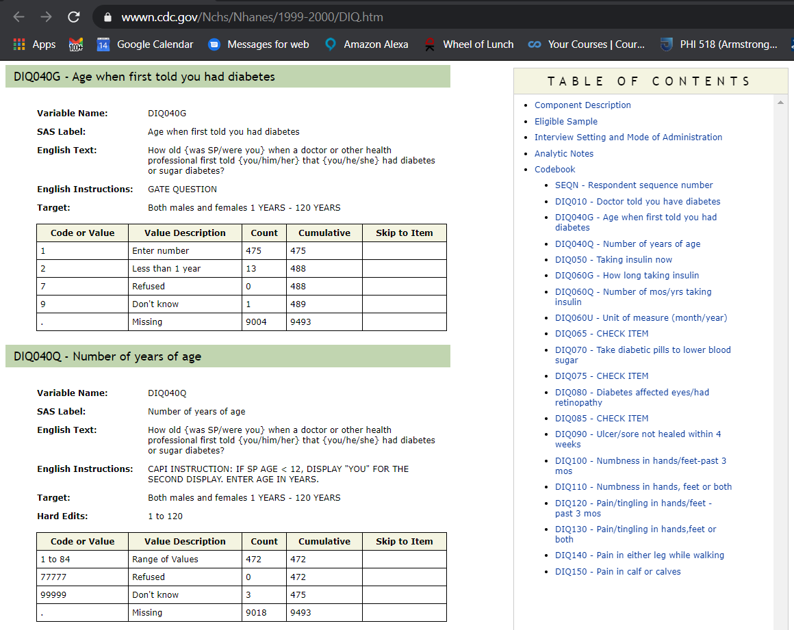

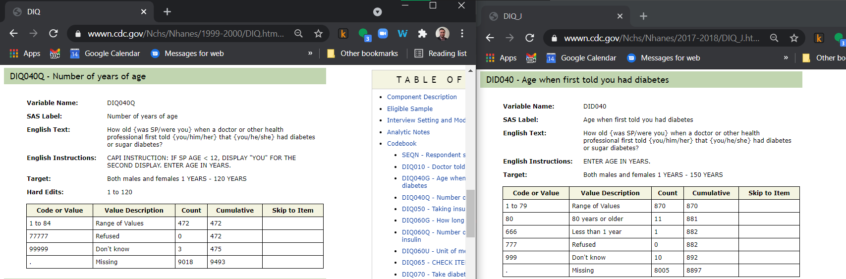
So when yr_range == 1991-2000 then AGE_AT_DIAG_DM2 will be equal to DIQ040Q. However, when DIQ040Q is between 1 and 84 that is the age number. When DIQ040Q is 77777, 99999 or missing we do not know the member’s age number so we might as well classify all of these as missing.

3.6.3 DIQ : Age at Diabetes : 2001-2004

The second range of years occurs over multiple year ranges. We might make use of the METADATA table to assist us with querying the DIQ table.

For instance notice the METADATA table has a start_yr and end_yr numerical inputs on the same line associated with yr_range which is on the DIQ table:

METADATA %>%
  filter(Valid_Table == 1) %>%
  filter(Table_Name == 'DIQ') %>%
  select(yr_range_int, yr_range, start_yr, end_yr, Table_Name) 
#> # Source:   lazy query [?? x 5]
#> # Database: sqlite 3.35.5
#> #   [C:\Users\jkyle\Documents\GitHub\Jeff_Data_Mgt_R_PRV\DATA\sql_db\NHANES_DB.db]
#>   yr_range_int yr_range  start_yr end_yr Table_Name
#>          <int> <chr>        <dbl>  <dbl> <chr>     
#> 1            1 1999-2000     1999   2000 DIQ       
#> 2            2 2001-2002     2001   2002 DIQ       
#> 3            3 2003-2004     2003   2004 DIQ       
#> 4            4 2005-2006     2005   2006 DIQ       
#> 5            5 2007-2008     2007   2008 DIQ       
#> 6            6 2009-2010     2009   2010 DIQ       
#> # ... with more rows

So we can utilize the start_yr and end_year of the METADATA table in relation to the DIQ table:

METADATA %>%
  filter(Valid_Table == 1) %>% # Where Valid_Table = 1 
  filter(Table_Name == "DIQ") %>% # where Table_Name  = 'DIQ'
  filter(2001 <= start_yr & end_yr <= 2004) %>% # where 2001 <= start_yr AND end_yr <= 2004
  select(yr_range) %>% # select yr_ranges
  inner_join(DIQ)  %>% # JOIN DIQ
  select(SEQN, yr_range, DIQ040G, DIQ040Q, DID040G, DID040Q, DID040) %>% # select columns of interest
  filter(!(is.na(DIQ040G) & is.na(DIQ040Q) & is.na(DID040G) &  is.na(DID040Q) & is.na(DID040))) %>% # one of these columns should be non-missing
  glimpse()
#> Joining, by = "yr_range"
#> Rows: ??
#> Columns: 7
#> Database: sqlite 3.35.5 [C:\Users\jkyle\Documents\GitHub\Jeff_Data_Mgt_R_PRV\DATA\sql_db\NHANES_DB.db]
#> $ SEQN     <dbl> 9988, 10004, 10005, 10007, 10101, 10104, 10106, 10131, 10163,~
#> $ yr_range <chr> "2001-2002", "2001-2002", "2001-2002", "2001-2002", "2001-200~
#> $ DIQ040G  <dbl> NA, NA, NA, NA, NA, NA, NA, NA, NA, NA, NA, NA, NA, NA, NA, N~
#> $ DIQ040Q  <dbl> NA, NA, NA, NA, NA, NA, NA, NA, NA, NA, NA, NA, NA, NA, NA, N~
#> $ DID040G  <dbl> 1, 1, 1, 1, 1, 1, 1, 1, 1, 1, 1, 1, 2, 1, 1, 1, 1, 1, 1, 1, 9~
#> $ DID040Q  <dbl> 40, 34, 38, 55, 56, 47, 55, 64, 35, 33, 45, 60, NA, 32, 37, 4~
#> $ DID040   <dbl> NA, NA, NA, NA, NA, NA, NA, NA, NA, NA, NA, NA, NA, NA, NA, N~

When 2001 <= start_yr & end_yr <= 2004 then DID040Q is the age number.

We have a couple more to check that are very similar to this.

We have two options as to how to proceed: 1. We can copy the above code 2x and modifying each one OR 2. we can make a helper function:

3.7 `AGE_AT_DIAG_VIEW` helper function

We might want to standardize the above view as as an R function.

Below we take in input start_year and end_year’s query the METADATA table for all valid DIQ tables between those values:

AGE_AT_DIAG_VIEW <- function(my_start_year, my_end_year){
  
  if(is.null(my_start_year) | is.null(my_end_year)){
    print("ERROR : my_start_year and my_end_year must be numeric int ( > 1998 and < 2018 ) \n")
  }
  
  tmp <- METADATA %>%
  filter(Valid_Table == 1) %>%
  filter(Table_Name == "DIQ") %>%
  filter(my_start_year <= start_yr & end_yr <= my_end_year) %>%
  select(yr_range) %>%
  inner_join(DIQ)  %>%
  select(SEQN, yr_range, DIQ040G, DIQ040Q, DID040G, DID040Q, DID040) %>%
  filter(!(is.na(DIQ040G) & is.na(DIQ040Q) & is.na(DID040G) &  is.na(DID040Q) & is.na(DID040))) 
  
  return( tmp )
}

Notice that writing this function amounts to replicating the code one time with the following changes:

create a function called AGE_AT_DIAG_VIEW with AGE_AT_DIAG_VIEW <- function(my_start_year, my_end_year){
we added some error checks on the inputs my_start_year and my_end_year
we added tmp assignment to our dplyr string we found above
replace 2001 with my_start_year
replace 2004 with my_end_year
we return tmp and close the function definition.

First, let’s test it against some output we already are familiar with:

AGE_AT_DIAG_VIEW(2001 , 2004) %>% 
  glimpse()
#> Joining, by = "yr_range"
#> Rows: ??
#> Columns: 7
#> Database: sqlite 3.35.5 [C:\Users\jkyle\Documents\GitHub\Jeff_Data_Mgt_R_PRV\DATA\sql_db\NHANES_DB.db]
#> $ SEQN     <dbl> 9988, 10004, 10005, 10007, 10101, 10104, 10106, 10131, 10163,~
#> $ yr_range <chr> "2001-2002", "2001-2002", "2001-2002", "2001-2002", "2001-200~
#> $ DIQ040G  <dbl> NA, NA, NA, NA, NA, NA, NA, NA, NA, NA, NA, NA, NA, NA, NA, N~
#> $ DIQ040Q  <dbl> NA, NA, NA, NA, NA, NA, NA, NA, NA, NA, NA, NA, NA, NA, NA, N~
#> $ DID040G  <dbl> 1, 1, 1, 1, 1, 1, 1, 1, 1, 1, 1, 1, 2, 1, 1, 1, 1, 1, 1, 1, 9~
#> $ DID040Q  <dbl> 40, 34, 38, 55, 56, 47, 55, 64, 35, 33, 45, 60, NA, 32, 37, 4~
#> $ DID040   <dbl> NA, NA, NA, NA, NA, NA, NA, NA, NA, NA, NA, NA, NA, NA, NA, N~

Now checking the remaining options will require far less code:

3.7.1 DIG : Age at Diabetes : 2005-2008

AGE_AT_DIAG_VIEW(2005 , 2008) %>%
  glimpse()
#> Joining, by = "yr_range"
#> Rows: ??
#> Columns: 7
#> Database: sqlite 3.35.5 [C:\Users\jkyle\Documents\GitHub\Jeff_Data_Mgt_R_PRV\DATA\sql_db\NHANES_DB.db]
#> $ SEQN     <dbl> 31132, 31151, 31162, 31186, 31194, 31233, 31257, 31307, 31311~
#> $ yr_range <chr> "2005-2006", "2005-2006", "2005-2006", "2005-2006", "2005-200~
#> $ DIQ040G  <dbl> NA, NA, NA, NA, NA, NA, NA, NA, NA, NA, NA, NA, NA, NA, NA, N~
#> $ DIQ040Q  <dbl> NA, NA, NA, NA, NA, NA, NA, NA, NA, NA, NA, NA, NA, NA, NA, N~
#> $ DID040G  <dbl> NA, NA, NA, NA, NA, NA, NA, NA, NA, NA, NA, NA, NA, NA, NA, N~
#> $ DID040Q  <dbl> NA, NA, NA, NA, NA, NA, NA, NA, NA, NA, NA, NA, NA, NA, NA, N~
#> $ DID040   <dbl> 63, 50, 40, 44, 44, 75, 50, 76, 61, 45, 56, 65, 55, 56, 40, 4~

When 2005 <= start_yr & end_yr <= 2008 then DID040 is the age number.

3.7.2 DIG : Age at Diabetes : 2009-2018

AGE_AT_DIAG_VIEW(2009 , 2018)
#> Joining, by = "yr_range"
#> # Source:   lazy query [?? x 7]
#> # Database: sqlite 3.35.5
#> #   [C:\Users\jkyle\Documents\GitHub\Jeff_Data_Mgt_R_PRV\DATA\sql_db\NHANES_DB.db]
#>    SEQN yr_range  DIQ040G DIQ040Q DID040G DID040Q DID040
#>   <dbl> <chr>       <dbl>   <dbl>   <dbl>   <dbl>  <dbl>
#> 1 51628 2009-2010      NA      NA      NA      NA     56
#> 2 51635 2009-2010      NA      NA      NA      NA     70
#> 3 51643 2009-2010      NA      NA      NA      NA     34
#> 4 51668 2009-2010      NA      NA      NA      NA     25
#> 5 51690 2009-2010      NA      NA      NA      NA     55
#> 6 51702 2009-2010      NA      NA      NA      NA     35
#> # ... with more rows

When 2009 <= start_yr & end_yr <= 2018 then DID040 is the age number.

3.8 Define `AGE_AT_DIAG_DM2`

Now that we have confirmed each of the columns that contain the age at which the member reports first having diabetes we are one step closer to defining the feature.

We know each of the age numbers has ranges of valid and invalid values that shifts year-to-year. We believe the following code can account for many of the individual data issues without great loss of data quality until a more through review of each tables can be performed:


AGE_AT_DIAG_DM2_TBL <- METADATA %>%
  filter(Valid_Table == 1) %>%
  filter(Table_Name == 'DIQ') %>%
  select(yr_range, start_yr, end_yr) %>%
  left_join(DIQ) %>%
  select(SEQN, yr_range, start_yr, end_yr, DIQ040G, DIQ040Q, DID040G, DID040Q, DID040) %>%
  mutate(AGE_AT_DIAG_DM2_1 = 
           case_when(1991 <= start_yr & end_yr <= 2000 ~ DIQ040Q,
                     2001 <= start_yr & end_yr <= 2004 ~ DID040Q,
                     2005 <= start_yr & end_yr <= 2018 ~ DID040)) %>% 
  mutate(AGE_AT_DIAG_DM2 = 
           case_when(is.na(AGE_AT_DIAG_DM2_1)  ~ NA , 
                     AGE_AT_DIAG_DM2_1 < 1 | 84 < AGE_AT_DIAG_DM2_1 ~ NA,
                     79 < AGE_AT_DIAG_DM2_1  & AGE_AT_DIAG_DM2_1 < 85 ~ 82,
                     0 < AGE_AT_DIAG_DM2_1 & AGE_AT_DIAG_DM2_1 < 80  ~ AGE_AT_DIAG_DM2_1)) %>%
  select(SEQN, AGE_AT_DIAG_DM2)
#> Joining, by = "yr_range"

In the first part of the query, from the METADATA to the select(SEQN, yr_range, start_yr, end_yr, DIQ040G, DIQ040Q, DID040G, DID040Q, DID040) %>% we are using the information we gathered from our helper function.

In the next mutate statement, we review the above information we gathered in applying the helper function and map DIQ040Q , DID040Q, and DID040 into AGE_AT_DIAG_DM2_1 by the proper corresponding start_yr and end_yr.

In the next mutate statement we make some educated guesses about the valid ranges of “Age at diagnosis”:

If it’s missing, it’s missing.
If it’s less then 1 or it’s greater than 84 it’s missing.
If the value is greater than 79 and less then 85 we will just average out the errors over time by using mean(79:85) = 82
Lastly, if the value is greater than 0 but less than 80 we will assume it was entered be the age at diagnosis of diabetes.

Lastly, we select only the information we need to avoid confusion.

Here’s a quick look at some non-missing values:

AGE_AT_DIAG_DM2_TBL %>% 
  filter(!is.na(AGE_AT_DIAG_DM2)) %>%
  glimpse()
#> Rows: ??
#> Columns: 2
#> Database: sqlite 3.35.5 [C:\Users\jkyle\Documents\GitHub\Jeff_Data_Mgt_R_PRV\DATA\sql_db\NHANES_DB.db]
#> $ SEQN            <dbl> 13, 29, 40, 55, 71, 83, 130, 148, 163, 187, 266, 272, ~
#> $ AGE_AT_DIAG_DM2 <dbl> 67, 61, 63, 57, 60, 57, 1, 76, 56, 66, 20, 19, 32, 60,~

\(~\)

3.9 Outcome Table

DEMO <- tbl(NHANES_DB, "DEMO")

OUTCOME_TBL <- DEMO %>% 
  select(SEQN) %>% 
  left_join(DM2_TBL) %>%
  left_join(AGE_AT_DIAG_DM2_TBL) 
#> Joining, by = "SEQN"
#> Joining, by = "SEQN"

\(~\)

3.10 Define Features - Gender and Age

Open_NHANES_table_help('DEMO')

INPUT_TBL <- DEMO %>%
  mutate(Gender = if_else(RIAGENDR == 2 , "Female", "Male")) %>%
  mutate(Age = if_else(is.na(RIDAGEYR), RIDAGEMN/12 , RIDAGEYR)) %>%
  select(SEQN, yr_range, Age, Gender) %>%
  glimpse()
#> Rows: ??
#> Columns: 4
#> Database: sqlite 3.35.5 [C:\Users\jkyle\Documents\GitHub\Jeff_Data_Mgt_R_PRV\DATA\sql_db\NHANES_DB.db]
#> $ SEQN     <dbl> 1, 2, 3, 4, 5, 6, 7, 8, 9, 10, 11, 12, 13, 14, 15, 16, 17, 18~
#> $ yr_range <chr> "1999-2000", "1999-2000", "1999-2000", "1999-2000", "1999-200~
#> $ Age      <dbl> 2, 77, 10, 1, 49, 19, 59, 13, 11, 43, 15, 37, 70, 81, 38, 85,~
#> $ Gender   <chr> "Female", "Male", "Female", "Male", "Male", "Female", "Female~

\(~\)

3.11 Analytic Data-Sets

An analytic data-set primarily consists of columns of targets and features to analyze the data or complete a prediction task.

Note there may be other useful columns that are assigned other roles in the predictive modeling tasks.

surrogate keys or other identifiers

example : SEQN is the surrogate key for a patient ID - each respondent has a unique SEQN

grouping or partitioning columns

example : yr_range the survey is taken in year ranges and there are some shifts year-to-year in column information

raw or source columns are also permitted

we might want to experiment with various definition of a feature “on-the-fly” so it might be helpful to keep some source information while we iterate on our analysis set.

Ultimately, The data science team is responsible to ensure all data-inputs into predictive models will be read as valid features, which will not heavily leak into the model prediction task. The goal of having analytic data-sets is to make analysis easier for researchers to understand and iterate on the overall data science pipeline.

3.12 Example

The Table A_DATA_TBL below is a simple example of an analytic data-set:


A_DATA_TBL <- INPUT_TBL %>%
  left_join(OUTCOME_TBL)
#> Joining, by = "SEQN"


A_DATA_TBL %>%
  glimpse()
#> Rows: ??
#> Columns: 6
#> Database: sqlite 3.35.5 [C:\Users\jkyle\Documents\GitHub\Jeff_Data_Mgt_R_PRV\DATA\sql_db\NHANES_DB.db]
#> $ SEQN            <dbl> 1, 2, 3, 4, 5, 6, 7, 8, 9, 10, 11, 12, 13, 14, 15, 16,~
#> $ yr_range        <chr> "1999-2000", "1999-2000", "1999-2000", "1999-2000", "1~
#> $ Age             <dbl> 2, 77, 10, 1, 49, 19, 59, 13, 11, 43, 15, 37, 70, 81, ~
#> $ Gender          <chr> "Female", "Male", "Female", "Male", "Male", "Female", ~
#> $ DIABETES        <dbl> 0, 0, 0, 0, 0, 0, 0, 0, 0, 0, 0, 0, 1, 0, 0, 0, 0, 0, ~
#> $ AGE_AT_DIAG_DM2 <dbl> NA, NA, NA, NA, NA, NA, NA, NA, NA, NA, NA, NA, 67, NA~

\(~\)

3.13 Example Summary Tables with `dplyr`:

3.13.1 Count of Diabetes

A_DATA_TBL %>%
  group_by(DIABETES) %>%
  summarise(n = n_distinct(SEQN))
#> # Source:   lazy query [?? x 2]
#> # Database: sqlite 3.35.5
#> #   [C:\Users\jkyle\Documents\GitHub\Jeff_Data_Mgt_R_PRV\DATA\sql_db\NHANES_DB.db]
#>   DIABETES     n
#>      <dbl> <int>
#> 1       NA  5769
#> 2        0 88740
#> 3        1  6807

A_DATA_TBL %>%
  group_by(DIABETES) %>%
  tally()
#> # Source:   lazy query [?? x 2]
#> # Database: sqlite 3.35.5
#> #   [C:\Users\jkyle\Documents\GitHub\Jeff_Data_Mgt_R_PRV\DATA\sql_db\NHANES_DB.db]
#>   DIABETES     n
#>      <dbl> <int>
#> 1       NA  5769
#> 2        0 88740
#> 3        1  6807

3.13.2 Average Age by Gender

A_DATA_TBL %>%
  group_by(Gender) %>%
  summarise(mean_Age = mean(Age))
#> Warning: Missing values are always removed in SQL.
#> Use `mean(x, na.rm = TRUE)` to silence this warning
#> This warning is displayed only once per session.
#> # Source:   lazy query [?? x 2]
#> # Database: sqlite 3.35.5
#> #   [C:\Users\jkyle\Documents\GitHub\Jeff_Data_Mgt_R_PRV\DATA\sql_db\NHANES_DB.db]
#>   Gender mean_Age
#>   <chr>     <dbl>
#> 1 Female     31.5
#> 2 Male       30.8

We see that R gives us a warning about what is happening with the NA values. If we want to let R know that we encourage this behavior we use:

A_DATA_TBL %>%
  group_by(Gender) %>%
  summarise(mean_Age = mean(Age, na.rm=TRUE))
#> # Source:   lazy query [?? x 2]
#> # Database: sqlite 3.35.5
#> #   [C:\Users\jkyle\Documents\GitHub\Jeff_Data_Mgt_R_PRV\DATA\sql_db\NHANES_DB.db]
#>   Gender mean_Age
#>   <chr>     <dbl>
#> 1 Female     31.5
#> 2 Male       30.8

3.13.3 Counts of Diabetic Status by Gender

A_DATA_TBL %>% 
  group_by(DIABETES, Gender) %>%
  tally() 
#> # Source:   lazy query [?? x 3]
#> # Database: sqlite 3.35.5
#> #   [C:\Users\jkyle\Documents\GitHub\Jeff_Data_Mgt_R_PRV\DATA\sql_db\NHANES_DB.db]
#> # Groups:   DIABETES
#>   DIABETES Gender     n
#>      <dbl> <chr>  <int>
#> 1       NA Female  2864
#> 2       NA Male    2905
#> 3        0 Female 45188
#> 4        0 Male   43552
#> 5        1 Female  3371
#> 6        1 Male    3436

We can also continue to use dplyr after a summary table; here we use pivot_wider which is in the tidyr library, here, pivot_wider is creating new column names from the discrete values in the Gender column (names_from = Gender), the values that populate those entries will come from the n in the tally this specified with the values_from = n below:

A_DATA_TBL %>% 
  group_by(DIABETES, Gender) %>%
  tally() %>%
  tidyr::pivot_wider(names_from = Gender , values_from = n)
#> # Source:   lazy query [?? x 3]
#> # Database: sqlite 3.35.5
#> #   [C:\Users\jkyle\Documents\GitHub\Jeff_Data_Mgt_R_PRV\DATA\sql_db\NHANES_DB.db]
#> # Groups:   DIABETES
#>   DIABETES Female  Male
#>      <dbl>  <int> <int>
#> 1       NA   2864  2905
#> 2        0  45188 43552
#> 3        1   3371  3436

3.13.4 Count of Female patients with Diabetes

A_DATA_TBL %>% 
  group_by(DIABETES, Gender) %>%
  tally() %>%
  filter(DIABETES == 1) %>%
  filter(Gender == "Female")
#> # Source:   lazy query [?? x 3]
#> # Database: sqlite 3.35.5
#> #   [C:\Users\jkyle\Documents\GitHub\Jeff_Data_Mgt_R_PRV\DATA\sql_db\NHANES_DB.db]
#> # Groups:   DIABETES
#>   DIABETES Gender     n
#>      <dbl> <chr>  <int>
#> 1        1 Female  3371

A_DATA_TBL %>%
  filter(DIABETES == 1) %>%
  filter(Gender == "Female") %>%
  tally() 
#> # Source:   lazy query [?? x 1]
#> # Database: sqlite 3.35.5
#> #   [C:\Users\jkyle\Documents\GitHub\Jeff_Data_Mgt_R_PRV\DATA\sql_db\NHANES_DB.db]
#>       n
#>   <int>
#> 1  3371

3.13.5 Counts and Mean Age of Member by Diabetic Status and Gender

Note that we can specify the .groups option in a summarise on a grouped dataframe the options are:

“keep”: Same grouping structure as the grouped data.
“drop_last”: dropping the last level of grouping.
“drop”: All levels of grouping are dropped.
“rowwise”: Each row is its own group

When .groups is not specified, it is chosen based on the number of rows of the results:

If all the results have 1 row, you get “drop_last.”
If the number of rows varies, you get “keep.”

A_DATA_TBL %>% 
  group_by(DIABETES, Gender) %>%
  summarise(n = n_distinct(SEQN),
            Mean_Age = mean(Age, na.rm=TRUE),
            .groups = 'keep')
#> # Source:   lazy query [?? x 4]
#> # Database: sqlite 3.35.5
#> #   [C:\Users\jkyle\Documents\GitHub\Jeff_Data_Mgt_R_PRV\DATA\sql_db\NHANES_DB.db]
#> # Groups:   DIABETES, Gender
#>   DIABETES Gender     n Mean_Age
#>      <dbl> <chr>  <int>    <dbl>
#> 1       NA Female  2864     12.1
#> 2       NA Male    2905     11.9
#> 3        0 Female 45188     30.5
#> 4        0 Male   43552     29.5
#> 5        1 Female  3371     61.1
#> 6        1 Male    3436     62.0

Again, we can reformat the table with pivot_wider - this time we will get values from both n and Mean_Age:

A_DATA_TBL %>% 
  group_by(DIABETES, Gender) %>%
  summarise(n = n_distinct(SEQN),
            Mean_Age = mean(Age, na.rm=TRUE),
            .groups = 'keep') %>%
  ungroup() %>%
  pivot_wider(names_from = Gender , values_from = c('n', 'Mean_Age'))
#> # Source:   lazy query [?? x 5]
#> # Database: sqlite 3.35.5
#> #   [C:\Users\jkyle\Documents\GitHub\Jeff_Data_Mgt_R_PRV\DATA\sql_db\NHANES_DB.db]
#>   DIABETES n_Female n_Male Mean_Age_Female Mean_Age_Male
#>      <dbl>    <int>  <int>           <dbl>         <dbl>
#> 1       NA     2864   2905            12.1          11.9
#> 2        0    45188  43552            30.5          29.5
#> 3        1     3371   3436            61.1          62.0

3.13.6 Average Age of Male with Diabetes

A_DATA_TBL %>% 
  group_by(DIABETES, Gender) %>%
  summarise(Mean_Age = mean(Age, na.rm=TRUE),
            .groups = 'keep') %>%
  filter(Gender == 'Male') %>%
  filter(DIABETES == 1)
#> # Source:   lazy query [?? x 3]
#> # Database: sqlite 3.35.5
#> #   [C:\Users\jkyle\Documents\GitHub\Jeff_Data_Mgt_R_PRV\DATA\sql_db\NHANES_DB.db]
#> # Groups:   DIABETES, Gender
#>   DIABETES Gender Mean_Age
#>      <dbl> <chr>     <dbl>
#> 1        1 Male       62.0

A_DATA_TBL  %>% 
  filter(Gender == 'Male') %>%
  filter(DIABETES == 1) %>%
  summarise(Mean_Age = mean(Age, na.rm=TRUE),
            .groups = 'keep') 
#> # Source:   lazy query [?? x 1]
#> # Database: sqlite 3.35.5
#> #   [C:\Users\jkyle\Documents\GitHub\Jeff_Data_Mgt_R_PRV\DATA\sql_db\NHANES_DB.db]
#>   Mean_Age
#>      <dbl>
#> 1     62.0

3.13.7 By Gender and Diabetic condition, how many patients are younger than average among their group?

Mean_Age.by_DM2_Gender <- A_DATA_TBL %>% 
  group_by(DIABETES, Gender) %>%
  summarise(n = n_distinct(SEQN),
            Mean_Age = mean(Age, na.rm=TRUE),
            .groups = 'keep')

A_DATA_TBL %>%
  left_join(Mean_Age.by_DM2_Gender) %>%
  filter(Age < Mean_Age) %>%
  group_by(DIABETES, Gender) %>%
  summarise(n = n_distinct(SEQN),
            .groups = 'keep')
#> Joining, by = c("Gender", "DIABETES")
#> # Source:   lazy query [?? x 3]
#> # Database: sqlite 3.35.5
#> #   [C:\Users\jkyle\Documents\GitHub\Jeff_Data_Mgt_R_PRV\DATA\sql_db\NHANES_DB.db]
#> # Groups:   DIABETES, Gender
#>   DIABETES Gender     n
#>      <dbl> <chr>  <int>
#> 1        0 Female 26041
#> 2        0 Male   25377
#> 3        1 Female  1507
#> 4        1 Male    1444

3.13.8 How many people are in the top quartile of Age?

Use the ntile function with n = 4 for “quartile” :

A_DATA_TBL %>%
  mutate(ntile_4 = ntile(Age,4)) %>%
  filter(ntile_4 == 4) %>%
  tally()
#> # Source:   lazy query [?? x 1]
#> # Database: sqlite 3.35.5
#> #   [C:\Users\jkyle\Documents\GitHub\Jeff_Data_Mgt_R_PRV\DATA\sql_db\NHANES_DB.db]
#>       n
#>   <int>
#> 1 25329

3.13.9 How many Males with Diabetes are in the bottom quartile of Age?

A_DATA_TBL %>%
  mutate(ntile_4 = ntile(Age,4)) %>%
  group_by(DIABETES, Gender, ntile_4) %>%
  tally() %>%
  ungroup() %>%
  filter(ntile_4 == 1) %>% 
  filter(Diabetes == 1) %>%
  filter(Gender == 'Male') %>%
  select(n)
#> # Source:   lazy query [?? x 1]
#> # Database: sqlite 3.35.5
#> #   [C:\Users\jkyle\Documents\GitHub\Jeff_Data_Mgt_R_PRV\DATA\sql_db\NHANES_DB.db]
#>       n
#>   <int>
#> 1    12

A_DATA_TBL %>%
  mutate(ntile_4 = ntile(Age,4)) %>%
  filter(ntile_4 == 1) %>% 
  filter(DIABETES == 1) %>%
  filter(Gender == 'Male') %>%
  tally() 
#> # Source:   lazy query [?? x 1]
#> # Database: sqlite 3.35.5
#> #   [C:\Users\jkyle\Documents\GitHub\Jeff_Data_Mgt_R_PRV\DATA\sql_db\NHANES_DB.db]
#>       n
#>   <int>
#> 1    12

A_DATA_TBL %>%
  mutate(ntile_4 = ntile(Age,4)) %>%
  group_by(DIABETES, Gender, ntile_4) %>%
  tally() %>%
  filter(ntile_4 == 1) %>% 
  filter(DIABETES == 1) %>%
  filter(Gender == 'Male')
#> # Source:   lazy query [?? x 4]
#> # Database: sqlite 3.35.5
#> #   [C:\Users\jkyle\Documents\GitHub\Jeff_Data_Mgt_R_PRV\DATA\sql_db\NHANES_DB.db]
#> # Groups:   DIABETES, Gender
#>   DIABETES Gender ntile_4     n
#>      <dbl> <chr>    <int> <int>
#> 1        1 Male         1    12

3.13.10 Cumulative Member count by `yr_range`

A_DATA_TBL %>%
  mutate(is_person = if_else(SEQN > 0 , 1 , 0 )) %>%
  group_by(yr_range) %>%
  summarise(n_mbrs_per_yr_range = sum(is_person), .groups = 'keep') %>%
  arrange(yr_range) %>%
  mutate(cum_mbrs = cumsum(n_mbrs_per_yr_range)) 
#> Warning: Missing values are always removed in SQL.
#> Use `SUM(x, na.rm = TRUE)` to silence this warning
#> This warning is displayed only once per session.
#> Warning: ORDER BY is ignored in subqueries without LIMIT
#> i Do you need to move arrange() later in the pipeline or use window_order() instead?
#> # Source:     lazy query [?? x 3]
#> # Database:   sqlite 3.35.5
#> #   [C:\Users\jkyle\Documents\GitHub\Jeff_Data_Mgt_R_PRV\DATA\sql_db\NHANES_DB.db]
#> # Groups:     yr_range
#> # Ordered by: yr_range
#>   yr_range  n_mbrs_per_yr_range cum_mbrs
#>   <chr>                   <dbl>    <dbl>
#> 1 1999-2000                9965     9965
#> 2 2001-2002               11039    11039
#> 3 2003-2004               10122    10122
#> 4 2005-2006               10348    10348
#> 5 2007-2008               10149    10149
#> 6 2009-2010               10537    10537
#> # ... with more rows

\(~\)

3.14 Data from Connections

Up until this point we have utilized dplyr and dbplyr to interface with a sqlite file.

Ultimately, R will be somewhat limited in what it can do only utilizing SQL connections to data-bases. Different data-bases will have different functionalities and slight variants of SQL; and what you are able to accomplish from a Tera-Data database might be different from what you can accomplish using a Spark or sqlite connection.

For instance, some window functions may not work as expected with our example sqlite database.

Learning these various technical challenges that accompanies each context arises from working within or between them.

Explicitly, notice that:

str(A_DATA_TBL, 1)
#> List of 2
#>  $ src:List of 2
#>   ..- attr(*, "class")= chr [1:4] "src_SQLiteConnection" "src_dbi" "src_sql" "src"
#>  $ ops:List of 4
#>   ..- attr(*, "class")= chr [1:3] "op_join" "op_double" "op"
#>  - attr(*, "class")= chr [1:5] "tbl_SQLiteConnection" "tbl_dbi" "tbl_sql" "tbl_lazy" ...

The object A_DATA_TBL is a connection to our SQLite database, not an R data-frame-tibble.

In fact, if we want the SQL we created along the way we can export it using the show_query function:

A_DATA_TBL %>%
  show_query()
#> <SQL>
#> SELECT `LHS`.`SEQN` AS `SEQN`, `yr_range`, `Age`, `Gender`, `DIABETES`, `AGE_AT_DIAG_DM2`
#> FROM (SELECT `SEQN`, `yr_range`, CASE WHEN (((`RIDAGEYR`) IS NULL)) THEN (`RIDAGEMN` / 12.0) WHEN NOT(((`RIDAGEYR`) IS NULL)) THEN (`RIDAGEYR`) END AS `Age`, `Gender`
#> FROM (SELECT `SEQN`, `SDDSRVYR`, `RIDSTATR`, `RIDEXMON`, `RIAGENDR`, `RIDAGEYR`, `RIDAGEMN`, `RIDAGEEX`, `RIDRETH1`, `RIDRETH2`, `DMQMILIT`, `DMDBORN`, `DMDCITZN`, `DMDYRSUS`, `DMDEDUC3`, `DMDEDUC2`, `DMDEDUC`, `DMDSCHOL`, `DMDMARTL`, `DMDHHSIZ`, `INDHHINC`, `INDFMINC`, `INDFMPIR`, `RIDEXPRG`, `RIDPREG`, `DMDHRGND`, `DMDHRAGE`, `DMDHRBRN`, `DMDHREDU`, `DMDHRMAR`, `DMDHSEDU`, `WTINT2YR`, `WTINT4YR`, `WTMEC2YR`, `WTMEC4YR`, `SDMVPSU`, `SDMVSTRA`, `SDJ1REPN`, `DMAETHN`, `DMARACE`, `WTMREP01`, `WTMREP02`, `WTMREP03`, `WTMREP04`, `WTMREP05`, `WTMREP06`, `WTMREP07`, `WTMREP08`, `WTMREP09`, `WTMREP10`, `WTMREP11`, `WTMREP12`, `WTMREP13`, `WTMREP14`, `WTMREP15`, `WTMREP16`, `WTMREP17`, `WTMREP18`, `WTMREP19`, `WTMREP20`, `WTMREP21`, `WTMREP22`, `WTMREP23`, `WTMREP24`, `WTMREP25`, `WTMREP26`, `WTMREP27`, `WTMREP28`, `WTMREP29`, `WTMREP30`, `WTMREP31`, `WTMREP32`, `WTMREP33`, `WTMREP34`, `WTMREP35`, `WTMREP36`, `WTMREP37`, `WTMREP38`, `WTMREP39`, `WTMREP40`, `WTMREP41`, `WTMREP42`, `WTMREP43`, `WTMREP44`, `WTMREP45`, `WTMREP46`, `WTMREP47`, `WTMREP48`, `WTMREP49`, `WTMREP50`, `WTMREP51`, `WTMREP52`, `WTIREP01`, `WTIREP02`, `WTIREP03`, `WTIREP04`, `WTIREP05`, `WTIREP06`, `WTIREP07`, `WTIREP08`, `WTIREP09`, `WTIREP10`, `WTIREP11`, `WTIREP12`, `WTIREP13`, `WTIREP14`, `WTIREP15`, `WTIREP16`, `WTIREP17`, `WTIREP18`, `WTIREP19`, `WTIREP20`, `WTIREP21`, `WTIREP22`, `WTIREP23`, `WTIREP24`, `WTIREP25`, `WTIREP26`, `WTIREP27`, `WTIREP28`, `WTIREP29`, `WTIREP30`, `WTIREP31`, `WTIREP32`, `WTIREP33`, `WTIREP34`, `WTIREP35`, `WTIREP36`, `WTIREP37`, `WTIREP38`, `WTIREP39`, `WTIREP40`, `WTIREP41`, `WTIREP42`, `WTIREP43`, `WTIREP44`, `WTIREP45`, `WTIREP46`, `WTIREP47`, `WTIREP48`, `WTIREP49`, `WTIREP50`, `WTIREP51`, `WTIREP52`, `yr_range`, `SIALANG`, `SIAPROXY`, `SIAINTRP`, `FIALANG`, `FIAPROXY`, `FIAINTRP`, `MIALANG`, `MIAPROXY`, `MIAINTRP`, `AIALANG`, `DMDFMSIZ`, `DMDBORN2`, `INDHHIN2`, `INDFMIN2`, `DMDHRBR2`, `RIDRETH3`, `RIDEXAGY`, `RIDEXAGM`, `DMQMILIZ`, `DMQADFC`, `DMDBORN4`, `AIALANGA`, `DMDHHSZA`, `DMDHHSZB`, `DMDHHSZE`, `DMDHRBR4`, `DMDHRAGZ`, `DMDHREDZ`, `DMDHRMAZ`, `DMDHSEDZ`, CASE WHEN (`RIAGENDR` = 2.0) THEN ('Female') WHEN NOT(`RIAGENDR` = 2.0) THEN ('Male') END AS `Gender`
#> FROM `DEMO`)) AS `LHS`
#> LEFT JOIN (SELECT `LHS`.`SEQN` AS `SEQN`, `DIABETES`, `AGE_AT_DIAG_DM2`
#> FROM (SELECT `LHS`.`SEQN` AS `SEQN`, `DIABETES`
#> FROM (SELECT `SEQN`
#> FROM `DEMO`) AS `LHS`
#> LEFT JOIN (SELECT `SEQN`, CASE
#> WHEN (`DIQ010` = 1.0) THEN (1.0)
#> WHEN (`DIQ010` = 2.0) THEN (0.0)
#> WHEN ((`DIQ010` != 1.0 OR `DIQ010` != 2.0)) THEN (NULL)
#> END AS `DIABETES`
#> FROM `DIQ`) AS `RHS`
#> ON (`LHS`.`SEQN` = `RHS`.`SEQN`)
#> ) AS `LHS`
#> LEFT JOIN (SELECT `SEQN`, CASE
#> WHEN (((`AGE_AT_DIAG_DM2_1`) IS NULL)) THEN (NULL)
#> WHEN (`AGE_AT_DIAG_DM2_1` < 1.0 OR 84.0 < `AGE_AT_DIAG_DM2_1`) THEN (NULL)
#> WHEN (79.0 < `AGE_AT_DIAG_DM2_1` AND `AGE_AT_DIAG_DM2_1` < 85.0) THEN (82.0)
#> WHEN (0.0 < `AGE_AT_DIAG_DM2_1` AND `AGE_AT_DIAG_DM2_1` < 80.0) THEN (`AGE_AT_DIAG_DM2_1`)
#> END AS `AGE_AT_DIAG_DM2`
#> FROM (SELECT `SEQN`, `yr_range`, `start_yr`, `end_yr`, `DIQ040G`, `DIQ040Q`, `DID040G`, `DID040Q`, `DID040`, CASE
#> WHEN (1991.0 <= `start_yr` AND `end_yr` <= 2000.0) THEN (`DIQ040Q`)
#> WHEN (2001.0 <= `start_yr` AND `end_yr` <= 2004.0) THEN (`DID040Q`)
#> WHEN (2005.0 <= `start_yr` AND `end_yr` <= 2018.0) THEN (`DID040`)
#> END AS `AGE_AT_DIAG_DM2_1`
#> FROM (SELECT `LHS`.`yr_range` AS `yr_range`, `start_yr`, `end_yr`, `SEQN`, `DIQ010`, `DIQ040G`, `DIQ040Q`, `DIQ050`, `DIQ060G`, `DIQ060Q`, `DIQ060U`, `DIQ070`, `DIQ080`, `DIQ090`, `DIQ100`, `DIQ110`, `DIQ120`, `DIQ130`, `DIQ140`, `DIQ150`, `DID040G`, `DID040Q`, `DID060G`, `DID060Q`, `DID040`, `DIQ220`, `DIQ160`, `DIQ170`, `DIQ180`, `DIQ190A`, `DIQ190B`, `DIQ190C`, `DIQ200A`, `DIQ200B`, `DIQ200C`, `DID060`, `DID070`, `DIQ230`, `DIQ240`, `DID250`, `DID260`, `DIQ260U`, `DID270`, `DIQ280`, `DIQ290`, `DIQ300S`, `DIQ300D`, `DID310S`, `DID310D`, `DID320`, `DID330`, `DID340`, `DID350`, `DIQ350U`, `DIQ360`, `DID341`, `DIQ172`, `DIQ175A`, `DIQ175B`, `DIQ175C`, `DIQ175D`, `DIQ175E`, `DIQ175F`, `DIQ175G`, `DIQ175H`, `DIQ175I`, `DIQ175J`, `DIQ175K`, `DIQ175L`, `DIQ175M`, `DIQ175N`, `DIQ175O`, `DIQ175P`, `DIQ175Q`, `DIQ175R`, `DIQ175S`, `DIQ175T`, `DIQ175U`, `DIQ175V`, `DIQ175W`, `DIQ275`, `DIQ291`, `DIQ175X`
#> FROM (SELECT `yr_range`, `start_yr`, `end_yr`
#> FROM (SELECT *
#> FROM `METADATA`
#> WHERE (`Valid_Table` = 1.0))
#> WHERE (`Table_Name` = 'DIQ')) AS `LHS`
#> LEFT JOIN `DIQ` AS `RHS`
#> ON (`LHS`.`yr_range` = `RHS`.`yr_range`)
#> ))) AS `RHS`
#> ON (`LHS`.`SEQN` = `RHS`.`SEQN`)
#> ) AS `RHS`
#> ON (`LHS`.`SEQN` = `RHS`.`SEQN`)

3.14.1 `collect` what you need

Often, it is needed to collect data into the R environment to perform more detailed analysis than the SQL is capable of. Unless you are working with sparklyr, many R modeling packages will require the input data to be an R data-frame.


A_DATA <- A_DATA_TBL %>% 
  collect()

Now check the str of A_DATA:


str(A_DATA)
#> tibble [101,316 x 6] (S3: tbl_df/tbl/data.frame)
#>  $ SEQN           : num [1:101316] 1 2 3 4 5 6 7 8 9 10 ...
#>  $ yr_range       : chr [1:101316] "1999-2000" "1999-2000" "1999-2000" "1999-2000" ...
#>  $ Age            : num [1:101316] 2 77 10 1 49 19 59 13 11 43 ...
#>  $ Gender         : chr [1:101316] "Female" "Male" "Female" "Male" ...
#>  $ DIABETES       : num [1:101316] 0 0 0 0 0 0 0 0 0 0 ...
#>  $ AGE_AT_DIAG_DM2: num [1:101316] NA NA NA NA NA NA NA NA NA NA ...

and we can see we have a dataframe-tibble as a result.

Notice, since we have downloaded a data-set of dimension:

dim(A_DATA)
#> [1] 101316      6

Additionally, notice we may not get useful information if we attempt to apply the dim function to A_DATA_TBL since A_DATA_TBL is not a dataframe:

dim(A_DATA_TBL)
#> [1] NA  6

We still may be able to replicate the information we are looking for with various dplyr queries to the SQL back-end:

# number of rows 
A_DATA_TBL %>%
  tally()
#> # Source:   lazy query [?? x 1]
#> # Database: sqlite 3.35.5
#> #   [C:\Users\jkyle\Documents\GitHub\Jeff_Data_Mgt_R_PRV\DATA\sql_db\NHANES_DB.db]
#>        n
#>    <int>
#> 1 101316

# number of columns
A_DATA_TBL %>% 
  colnames() %>% 
  length()
#> [1] 6

3.15 Save Week 2 Analysis Data

We will save the data-frame for the moment and continue our investigation.


A_DATA %>%
  saveRDS('C:/Users/jkyle/Documents/GitHub/Jeff_Data_Wrangling/Week_2/DATA/A_DATA.RDS')

3.16 Known sqlite limitations

Remark thus far my attempts to provide a bad window function example per have been fruit-less thus far, however, I have found it doesn’t like all join types:


ERROR <- DM2_TBL %>%
  full_join(AGE_AT_DIAG_DM2_TBL)
#> Joining, by = "SEQN"

ERROR %>% glimpse()
#> Rows: ??
#> Columns: 3
#> Database: sqlite 3.35.5 [C:\Users\jkyle\Documents\GitHub\Jeff_Data_Mgt_R_PRV\DATA\sql_db\NHANES_DB.db]
#> $ SEQN            <dbl> 1, 2, 3, 4, 5, 6, 7, 8, 9, 10, 11, 12, 13, 14, 15, 16,~
#> $ DIABETES        <dbl> 0, 0, 0, 0, 0, 0, 0, 0, 0, 0, 0, 0, 1, 0, 0, 0, 0, 0, ~
#> $ AGE_AT_DIAG_DM2 <dbl> NA, NA, NA, NA, NA, NA, NA, NA, NA, NA, NA, NA, 67, NA~

Remark we have already seen additional R functions that will “not translate to SQL” for example the hist function:


hist(A_DATA$AGE_AT_DIAG_DM2,
      main = "Histogram of Age at Diabetes",
      xlab = "Age at Diabetes")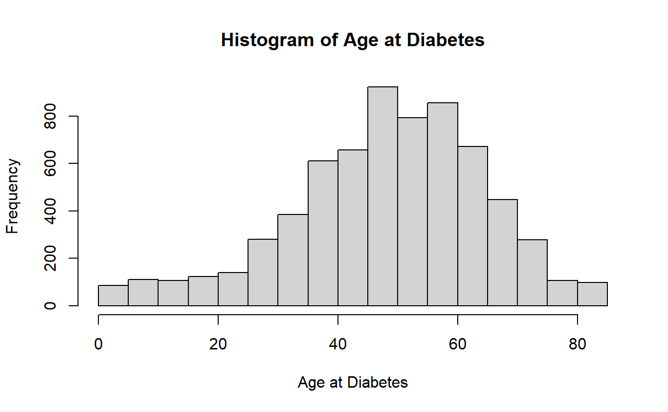


hist(A_DATA_TBL$AGE_AT_DIAG_DM2 ,
      main = "Histogram of Age at Diabetes",
      xlab = "Age at Diabetes")
#> Error in hist.default(A_DATA_TBL$AGE_AT_DIAG_DM2, main = "Histogram of Age at Diabetes", : 'x' must be numeric

However, we can still use R to a connected source without downloading large amounts of data:


hist( (A_DATA_TBL %>% select(AGE_AT_DIAG_DM2) %>% collect())$AGE_AT_DIAG_DM2 ,
      main = "Histogram of Age at Diabetes",
      xlab = "Age at Diabetes")

For instance if we wanted this graph:

A_DATA %>%
  filter(!is.na(DIABETES)) %>%
  mutate(DIABETES_factor = as.factor(DIABETES)) %>%
  ggplot(aes(x=Age, fill=DIABETES_factor)) +
  geom_density() + 
  labs(title = "Density Plot - Diabetes by Age")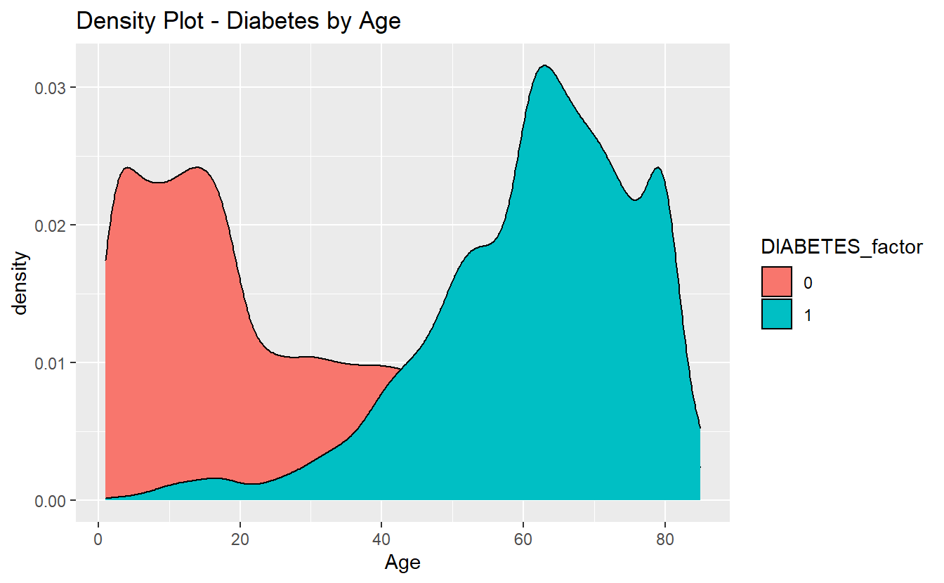

without having to download all of the data, we could do something like:

A_DATA_TBL %>%
  filter(!is.na(DIABETES)) %>%
  select(DIABETES, Age) %>% # select needed variables 
  collect() %>%  # collect only the data we want 
  mutate(DIABETES_factor = as.factor(DIABETES)) %>% #as.factor is an r function, SQLlite doesn't have "factor data type"
  ggplot(aes(x=Age, fill=DIABETES_factor)) +
  geom_density() + 
  labs(title = "Density Plot - Diabetes by Age")

3 Feature Engineering

3.1 Features and Targets

3.2 Example : Diabetes

3.3 Features and Targets Vary by Prediction Task.

3.3.1 Example : Depression

3.4 Define Targets - Diabetes and Age at Diabetes

3.5 Diabetes

3.6 Age at Diabetes

3.6.1 Analytic Notes on DIQ

3.6.2 DIQ : Age at Diabetes : 1991-2000

3.6.3 DIQ : Age at Diabetes : 2001-2004

3.7 AGE_AT_DIAG_VIEW helper function

3.7.1 DIG : Age at Diabetes : 2005-2008

3.7.2 DIG : Age at Diabetes : 2009-2018

3.8 Define AGE_AT_DIAG_DM2

3.9 Outcome Table

3.10 Define Features - Gender and Age

3.11 Analytic Data-Sets

3.12 Example

3.13 Example Summary Tables with dplyr:

3.13.1 Count of Diabetes

3.13.2 Average Age by Gender

3.13.3 Counts of Diabetic Status by Gender

3.13.4 Count of Female patients with Diabetes

3.13.5 Counts and Mean Age of Member by Diabetic Status and Gender

3.13.6 Average Age of Male with Diabetes

3.13.7 By Gender and Diabetic condition, how many patients are younger than average among their group?

3.13.8 How many people are in the top quartile of Age?

3.13.9 How many Males with Diabetes are in the bottom quartile of Age?

3.13.10 Cumulative Member count by yr_range

3.14 Data from Connections

3.14.1 collect what you need

3.15 Save Week 2 Analysis Data

3.16 Known sqlite limitations

3.7 `AGE_AT_DIAG_VIEW` helper function

3.8 Define `AGE_AT_DIAG_DM2`

3.13 Example Summary Tables with `dplyr`:

3.13.10 Cumulative Member count by `yr_range`

3.14.1 `collect` what you need