Multiple regression
Data Analytics Module
Lecturer: Hans van der Zwan
Handout 05
Topic: multiple regression
Literature
Rumsey D. J. (2010). Statistical Essentials for Dummies. Hoboken: Wiley Publishing.
Ismay C. & Kim A. Y. (2019). ModernDive. Statistical Inference for Data Science. https://moderndive.com.
Recommended literature
Preparation class
Watch: https://www.youtube.com/watch?v=dQNpSa-bq4M;
multiple regression (20 min.)
5 Multiple linear regression
A simple linear regression model is a model with a numeric Y-variable and one X-variable. Such a model can be easily expanded to a multiple reression model, i.e. a model with more than one X-variable. Assessing such a model doesn’t differ from assessing a simple linear regression model.
5.1 Multiple linear regression, an example
The buyer of a new car has to pay a special tax. The heigth of this special tax depends on different factors. Aim of this example is to find a model with which the heigth of the special tax for a Toyota can be estimated, based on different characteristics of this car. For this reason a random sample from in the Netherlands registered Toyota’s, has been drawn, reference date 2019-06-12; see file toyota_sample.csv.
5.1.1 Data description
The sample contains 400 observations on 15 variables.
As a first analysis the correlation coefficients between some of the numeric variables has been calculated. MS Excel: Data/Data Analysis/Correlation.
Figure 1
Correlation matrix generated with MS Excel

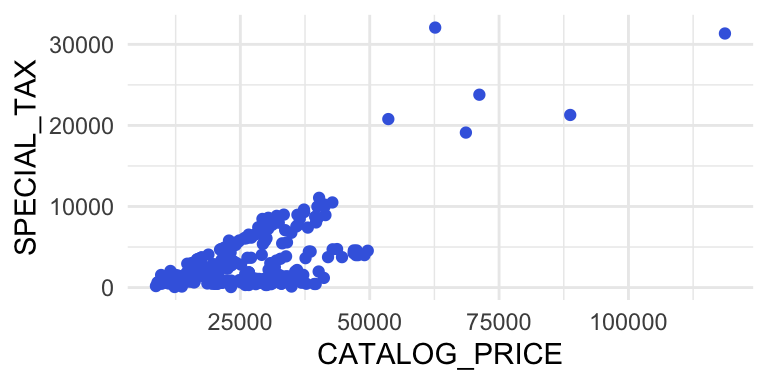
As can be seen in Figure 5 the variable SPECIAL_TAX has the highest correlation with CATALOG_PRICE. That’s why the first regression model is a simple linear refgression model with CATALOG_PRICE as explanatory variable.
Figure2
Scatterplot, SPECIAL_TAX in euro against CATALOG_PRICE in euro

5.1.2 Simple linear models
A first model uses CATALOG_PRICE as explanatory variable.
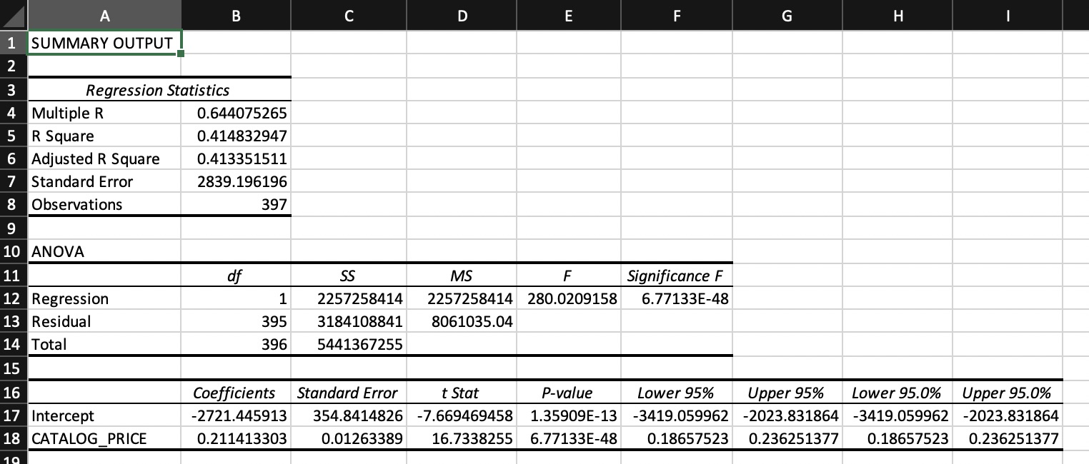
Figure 3
Excel output simple linear regression model

Note. MS Excel output simple linear regression model with SPECIAL_TAX as response variable and CATALOG_PRICE as explanatory variable. In the data file for three observations the catalog price is not available (NA), these observations have to be removed from the data to generate the regression model with Excel.
In this model R\(^2\) equals 0.415, so 41.5% of the variation in the catalog prices is explained by the model. Catalog price is a very significant variable in this model, p < .001. The value of the standard error of the estimate is 2839, i.e. 104.9% of the average SPECIAL-TAX values. This means that, although the variable is a significant explanatory variable, the model is not very usefull as a predcitive model.
A second model uses MASS as explanatory variable.
Figure 4
Excel output simple linear regression model
 Note. MS Excel output simple linear regression model with SPECIAL_TAX as response variable and MASS as explanatory variable.
In this model R\(^2\) equals 0.307, so 30.7% of the variation in the special tax values is explained by the model. Mass is a very significant variable in this model, p < .001. The standard error of the estimate is greater than in the first model. So overall this model is less good than the first model.
5.1.3 Multiple linear model (1) SPECIAL_TAX ~ MASS + CATALOG_PRICE
In a third model two explanatory variables ares used: MASS and CATALOG_PRICE. This model is sometimes notated as: SPECIAL_TAX ~ MASS + CATALOG_PRICE.
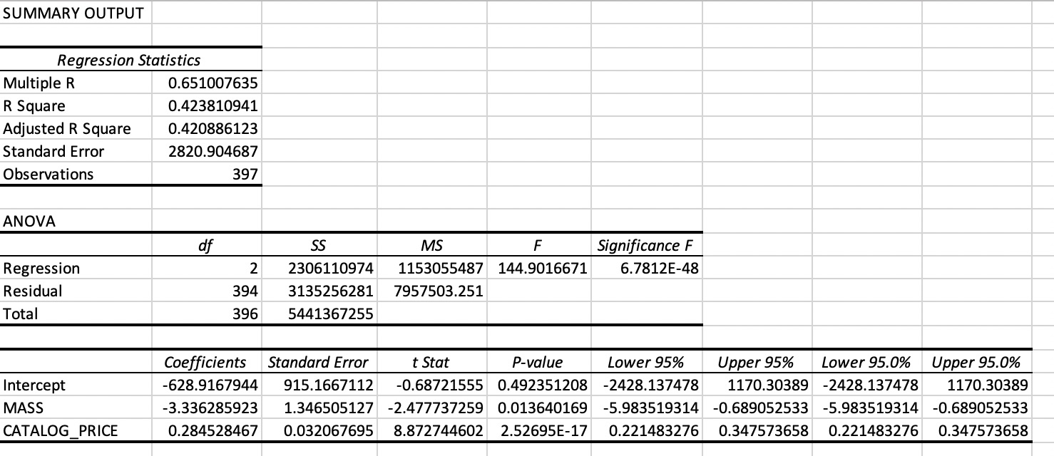
Figure 5
A multiple linear regression model
 Note. MS Excel output linear regression model with SPECIAL_TAX as response variable and CATALOG_PRICE and MASS as explanatory variables.
Although this model uses two explanatory variables which are both moderately correlated with the response variable SPECIAL_TAX, the model is not much better than the simple linear models, as can be seen by comparing the R\(^2\) values. The reason for this is that the two explanatory variables are highly correlated with each other. In general, it is preferable to use explanatory variables which are not correlated to each other.
Note that the coefficient of MASS in this model is even negative; so accoring to this model, with CATALOG_PRICE held fixed, the effect of MASS on CATALOG_PRICE is negative. Probalby the effect of MASS on is SPECIAL_TAX is mediated through CATALOG_PRICE, see section about Mediation Analysis.
5.1.4 Multiple linear model (2): SPECIAL_TAX ~ CATALOG_PRICE + ELECTRIC
The third model makes use of a dummy variable ELECTRIC (1 = FUEL_DESCRPTION=“ELECTRICITY”, 0 = FUEL_DESCRPTION<>“ELECTRICITY”).
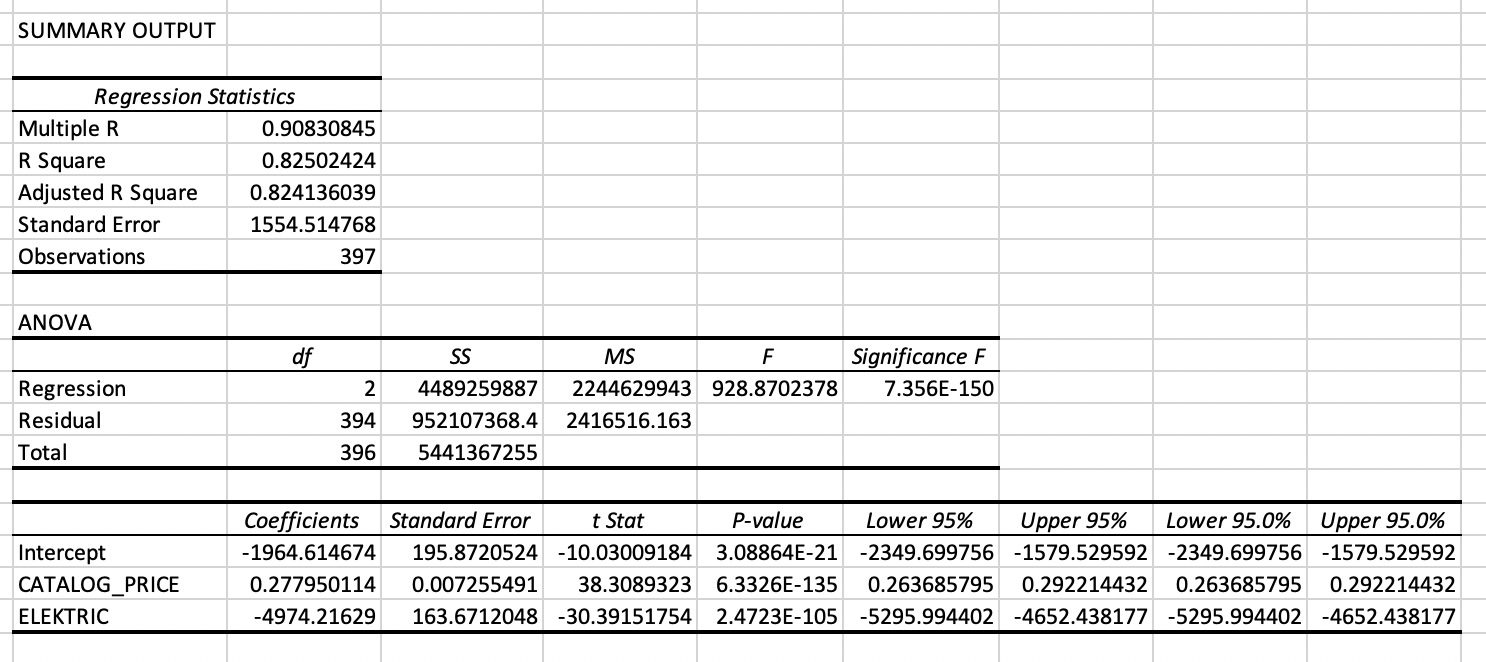
Figure 6
A multiple linear regression model
 Note. MS Excel output linear regression model with SPECIAL_TAX as response variable and CATALOG_PRICE and ELECTRIC as explanatory variables. ELECTRIC is a dummy variable which takes on value 1 if the car is an electric car and 0 otherwise.
This model is really an improvement of the simple regression model with CATALOG_PRICE as the only explanatory variable.
5.2 Panel Data Regression
The term Panel Data Analysis refers to a longitudinal study in which a couple of variabes are measured on the same object on different points in time. For instance an analysis of the development of the Life Expectancy per capita in different countries in relation to variables GDP per capita and Level of Education.
A multiple OLS regression model is not the best choice in such a case, because one of the assumptions for such a model is the independency of the observations. With longitudinal data, this assumption will be violated, because there might most probably be a dependency between the observations on the same object in the different time-periods.
That’s why in a regression model for panel data analysis, the time effect should be considered as well. For these cases there are different models applicable, depending on the specific context. Discussing these topics is beyond the scope of this course.
5.3 Mediation Regression Analysis
Mediation analysis is another application of regression analysis. In this case a situation is studied in which one variable affects a second variable that, in turn, affects a third variable.
As an example think of house prices as response variable and number of rooms and total area as explanatory variables. The effect of the number of rooms on the house price can be seen as mediated by the total area variable:
Number of Rooms –> Total Area –> House Price
Although normally using correlated X-variables in a multiple linear reggression model is considered to be a bad idea, in the case of mediation analysis the X-variables are related and the model is used to divide the effect of an X-variable on the Y-variable in an indirect effect - the effect via the mediator variable - and the direct effect.
For an introduciton to mediation analysis see for instance Kenny (2018).