Chapter 8 Text Analysis
Although the bulk of this guidebook is focused on quantitative analysis, the majority of the data in the real world is qualitative. The phone call you just had with a family member, the meetings you have with your peers and colleagues, as well as the thoughts you carry within you can be represented qualitatively. In fact, this tends to happen frequently whether you are aware of the process or not. When you call your health insurance company to and the automated operator asks you to state the reason for your call, you are logging qualitative data. When you end a zoom meeting a transcript is automatically created that lists all the words shared.
Words are an important part of the scientific method, so much so there has been a notable shift in many social sciences towards qualitative research methods. This chapter does not aim to present a breakdown of qualitative research methods. However, this chapter will provide you with an introduction to R packages and functions that assist in the process of text identification, manipulation, and analysis.
This chapter will utilize far more libraries than previous chapters, so it may be helpful to install each of the following packages at the onset.
library(tm) # a text mining package
library(stopwords)
library(tidytext) # a tidyverse friendly text mining package
library(stringr) # a package for manipulating strings
library(gutenbergr)
library(SnowballC) # a package for plotting text based data
library(wordcloud) # another package for plotting text data
library(lubridate)
library(tidyverse)
library(harrypotter) # contains a labelled  corpus of all harry potter books
library(sentimentr) # simple sentiment analysis function
library(textdata) # another package to support parsing
library(topicmodels) # specify, save and load topic models
library(LDAvis) # visualize the output of Latent Dirichlet Allocation
library(servr) # we use this library to access a data set
library(stringi) # natural language processing tools
library(ldatuning) # automatically specify LDA models
library(reshape2)
library(igraph)
library(ggraph)
devtools::install_github("bradleyboehmke/harrypotter")
8.1 R and Text Data
We have encountered text data previously as the “character” data type. The fundamental marker of “character” data is that these data are non-numeric. Character data types are referred to as “strings” individually. Any value inside double or single quotes is stored as a string. In the example below, the string “So long and thanks for all the fish” is input and received as output, while “So sad that it should come to this” is assigned to the object sv1 which can be recalled for future use.
"So long and thanks for all the fish"## [1] "So long and thanks for all the fish"sv1 <- "So sad that it should come to this"
sv1## [1] "So sad that it should come to this"Strings delineated by commas can also be assigned to objects as a vector. Run the following chunk to see how each word is separated into distinct strings.
sv2 <- c("We", "tried", "to", "warn", "you", "all", "but", "oh", "dear!")
sv2
## [1] "We" "tried" "to" "warn" "you" "all" "but" "oh" "dear!"When a string is included in a vector, R will assign other instances in that vector the string datatype. See the vector created below including multiple datatypes—including Boolean responses, strings, and numerical data. When we run the class function, everything was stored in quotes. As such, it is important to remember that if there is text data in a column, the rest of the column will be labelled as string data.
sv3 <- c("The world's about to be destroyed", TRUE, (1:7),
         "There's no point getting all annoyed", FALSE)
sv3
## [1] "The world's about to be destroyed"
## [2] "TRUE"
## [3] "1"
## [4] "2"
## [5] "3"
## [6] "4"
## [7] "5"
## [8] "6"
## [9] "7"
## [10] "There's no point getting all annoyed"
## [11] "FALSE"class(sv3)## [1] "character"length(sv3)## [1] 11To create a list of empty strings, use the character() function.
sv4 <- character(5)
sv4
## [1] "" "" "" "" ""class(sv4)## [1] "character"length(sv4)## [1] 5You can assign text within empty strings by calling the index and assigning it the desired text.
sv4[1] <- "first" # Add strings to a vector using its index
sv4
## [1] "first" "" "" "" ""Matrices also coerce numerical values to the characters. Use the
class() function to see the data type.
string_matrix <- rbind(1:5, letters[1:5])
string_matrix
## [,1] [,2] [,3] [,4] [,5]
## [1,] "1" "2" "3" "4" "5"
## [2,] "a" "b" "c" "d" "e"class(string_matrix[1,]) ## [1] "character"Dataframes, however, allow columns to retain data type independent of
the data type of other columns. Here, we created a new dataframe called
df, including the variables Sex, Name, and Age. See the structure of
the data frame below.
df <- data.frame("Sex" = 1:2, "Age" = c(21,15,18,22,19,23,21,22),
                 "Name" = c("John",
                            "Emily",
                            "Sam",
                            "Eleanor",
                            "Jonathan",
                            "Sarah",
                            "Ren",
                            "Jessie"))

str(df)
## 'data.frame': 8 obs. of 3 variables:
## $ Sex : int 1 2 1 2 1 2 1 2
## $ Age : num 21 15 18 22 19 23 21 22
## $ Name: chr "John" "Emily" "Sam" "Eleanor" ...The name column was assigned to be a factor as to retain levels for
subsequent analysis. Factors are the data objects which are used to
categorize the data and store it as levels. R may detects some strings
as a factors automatically. Use stringsAsFactors = False to avoid
this. There are cases in which it makes sense for strings to serve as
factors, for instance when categorical data are reported in a string
format.
df$Name <- as.factor(df$Name)
str(df)
## 'data.frame': 8 obs. of 3 variables:
## $ Sex : int 1 2 1 2 1 2 1 2
## $ Age : num 21 15 18 22 19 23 21 22
## $ Name: Factor w/ 8 levels "Eleanor","Emily",..: 4 2 7 1 5 8 6 3You can also use is.character() to assess whether a vector includes
character data or not.
df1 <- data.frame("Sex" = 1:2, "Age" = c(21,15,18,22,19,23,21,22),
"Name" = c("John", "Emily", "Sam", "Eleanor", "Jonathan","Sarah","Ren","Jessie"), stringsAsFactors = FALSE)

str(df1)
## 'data.frame': 8 obs. of 3 variables:
## $ Sex : int 1 2 1 2 1 2 1 2
## $ Age : num 21 15 18 22 19 23 21 22
## $ Name: chr "John" "Emily" "Sam" "Eleanor" ...is.character(df1$Name) ## [1] TRUE# Can also use is.character() function to tell if something has type "character"8.2 Cleaning and Processing Text
You can match and replace patterns using str_replace(), which searches
for matches to the argument (assigned object ‘pattern’) within character
vectors.
For larger text mining tasks, such as web scraping, you might use regular expressions, which is often shorted to regex. Regex allows you to construct string searching algorithms to find and replace very specific strings patterns that are not limited to literal characters (e.g. all four letter words in a data set).
Here’s a regex cheat sheet: http://www.rstudio.com/wp-content/uploads/2016/09/RegExCheatsheet.pdf. Additionally, you can search for and test regex text patterns here: https://regexr.com/
For our example, let’s create a string object that includes some unwanted noise.
sometext <- "I pulled /t/t/t/n/t/t some  weirdly /n/n formatted and encoded data from the internet and I want it/n/n/t/t/t/t/t/t to look cleaner./n/n"
sometext
## [1] "I pulled /t/t/t/n/t/t some weirdly /n/n formatted and encoded data from the internet and I want it/n/n/t/t/t/t/t/t to look cleaner./n/n"The str_detect() function searches for a character pattern in a
string: str_detect(pattern, string).
str_detect(sometext, "I pushed") ## [1] FALSEstr_detect(sometext, "I pulled") ## [1] TRUEThe str_replace_all() function finds and replaces a character pattern:
gsub(pattern, replacement, string). By running the following lines of
code, we will be able to replace instances of /t and /n with no data,
effectively deleting these. We will also delete a few instances of
double spaces with single space replacements.
sometext <- str_replace_all(sometext, "/t", "")
sometext <- str_replace_all(sometext, "/n", "")
sometext <- str_replace_all(sometext, "  ", " ")
sometext
## [1] "I pulled some weirdly formatted and encoded data from the internet and I want it to look cleaner."You can also use gsub() to include several replacements in the same
function separated by |. This code follows the same process as the
previous chunk.
sometext <- "I pulled /t/t/t/n/t/t some  weirdly /n/n formatted and encoded data from the internet and I want it/n/n/t/t/t/t/t/t to look cleaner./n/n"
spacingisoff <- gsub("/t|/n", "", sometext)
finaltext <- gsub("  ", " ", spacingisoff)
finaltext
## [1] "I pulled some weirdly formatted and encoded data from the internet and I want it to look cleaner."8.2.1 Case Study 1
For the first case study, we are going to use a collection of scraped Donald Trump tweets. Run each line in this chunk to load the data set from an OSF static link. Choose your own way to examine the data before we work with it.
load(url("https://osf.io/dvrhc/download"))
head(trumptweets$text)
## [1] "Just met with UN Secretary-General António Guterres who is working hard to “Make the United Nations Great Again.” When the UN does more to solve conflicts around the world, it means the U.S. has less to do and we save money. @NikkiHaley is doing a fantastic job! https://t.co/pqUv6cyH2z"
## [2] "America is a Nation that believes in the power of redemption. America is a Nation that believes in second chances - and America is a Nation that believes that the best is always yet to come! #PrisonReform https://t.co/Yk5UJUYgHN"
## [3] "RT @SteveForbesCEO: .@realDonaldTrump speech on drug costs pays immediate dividends. New @Amgen drug lists at 30% less than expected. Middl…"
## [4] "We grieve for the terrible loss of life, and send our support and love to everyone affected by this horrible attack in Texas. To the students, families, teachers and personnel at Santa Fe High School – we are with you in this tragic hour, and we will be with you forever... https://t.co/LtJ0D29Hsv"
## [5] "School shooting in Texas. Early reports not looking good. God bless all!"
## [6] "Reports are there was indeed at least one FBI representative implanted, for political purposes, into my campaign for president. It took place very early on, and long before the phony Russia Hoax became a “hot” Fake News story. If true - all time biggest political scandal!"The tidytext unnest() function pulls out tokens, or particular
words in a data set, from the column “text” and distributes them into
individual rows with accompanying metadata. Tokens represent individual
units of meaning, thus the process of dividing text data into individual
units is called ‘tokenization.’
In reading the code below, we are assigning a new object tidy_trumps
from the trumptweets dataset where %>% the columns created_at, text,
is_retweet, source, and hastags are isolated from the rest of the data
using select(), where then %>% the unnest_tokens() function is
deployed on the ‘text’ column at the word level. This argument can
also take sentence, ngram, and a few other options for dividing your
text data.
tidy_trumps <- trumptweets %>%
  select(created_at, text, is_retweet, source, hashtags) %>%
  unnest_tokens("word", text)

head(tidy_trumps)
## # A tibble: 6 × 5
## created_at is_retweet source hashtags word
## <dttm> <lgl> <chr> <list> <chr>
## 1 2018-05-18 20:41:21 FALSE Twitter for iPhone <chr [1]> just
## 2 2018-05-18 20:41:21 FALSE Twitter for iPhone <chr [1]> met
## 3 2018-05-18 20:41:21 FALSE Twitter for iPhone <chr [1]> with
## 4 2018-05-18 20:41:21 FALSE Twitter for iPhone <chr [1]> un
## 5 2018-05-18 20:41:21 FALSE Twitter for iPhone <chr [1]> secretary
## 6 2018-05-18 20:41:21 FALSE Twitter for iPhone <chr [1]> generalStop words are a set of commonly used words in a language. In natural
language processing, we want to filter these words from our data sets.
First, let’s examine the list of stop words from the tidytext package.
The lexicon refers to the source of the stop word, as this data set was
aggregated from three separate lists. (For more information, see the
link: https://juliasilge.github.io/tidytext/reference/stop_words.html)
data("stop_words")
head(stop_words)
## # A tibble: 6 × 2
## word lexicon
## <chr> <chr>
## 1 a SMART
## 2 a's SMART
## 3 able SMART
## 4 about SMART
## 5 above SMART
## 6 according SMARTWe can use the anti_join() function to tell R to find the stop words
in our list of tokens and remove them. This action is predicated on the
logic of joins, where data sets can be combined in a number of ways. The
removal of one token because it exists in another data set is a common
NLP task.
tidy_trumps <- tidy_trumps %>% anti_join(stop_words) ## Joining, by = "word"head(tidy_trumps)## # A tibble: 6 × 5
## created_at is_retweet source hashtags word
## <dttm> <lgl> <chr> <list> <chr>
## 1 2018-05-18 20:41:21 FALSE Twitter for iPhone <chr [1]> met
## 2 2018-05-18 20:41:21 FALSE Twitter for iPhone <chr [1]> secretary
## 3 2018-05-18 20:41:21 FALSE Twitter for iPhone <chr [1]> antónio
## 4 2018-05-18 20:41:21 FALSE Twitter for iPhone <chr [1]> guterres
## 5 2018-05-18 20:41:21 FALSE Twitter for iPhone <chr [1]> hard
## 6 2018-05-18 20:41:21 FALSE Twitter for iPhone <chr [1]> unitedUse the count() function to see a count of all tokens. The output is
not optimal, however. Sorting as TRUE doesn’t help much either.
head(tidy_trumps %>% count(word, sort = TRUE))## # A tibble: 6 × 2
## word n
## <chr> <int>
## 1 https 1281
## 2 t.co 1258
## 3 amp 562
## 4 rt 351
## 5 people 302
## 6 news 271If prevalent words in the data do not have practical meaning, we need to
eliminate their influence. You can create a custom table for the rest of
the words you’d like to omit using the code below using the
data.frame() function.
new_stop_words <- data.frame("word" = c("https", "t.co", "rt", "amp"), stringsAsFactors = FALSE)
str(new_stop_words)
## 'data.frame': 4 obs. of 1 variable:
## $ word: chr "https" "t.co" "rt" "amp"Now use the anti_join() to remove your new list of words and examine
readability of the output.
tidy_trumps <- tidy_trumps %>% anti_join(new_stop_words)## Joining, by = "word"head(tidy_trumps %>% count(word, sort = FALSE))## # A tibble: 6 × 2
## word n
## <chr> <int>
## 1 0 10
## 2 00 33
## 3 00am 1
## 4 00ame 1
## 5 00mao6vk7r 1
## 6 00pm 2As we recently saw, there are several numbers we need to get rid of in
the data. Let’s use grep and the regular expression for all digits for
this task. By the way, when we tokenized the text all punctuation was
removed thanks to tidytext.
tidy_trumps <- tidy_trumps[-grep("\\(?[0-9,.]+\\)?", tidy_trumps$word),]
tidy_trumps %>% count(word, sort = TRUE)
## # A tibble: 6,695 × 2
## word n
## <chr> <int>
## 1 people 302
## 2 news 271
## 3 president 235
## 4 fake 234
## 5 trump 218
## 6 country 213
## 7 america 204
## 8 tax 190
## 9 time 173
## 10 american 171
## # … with 6,685 more rowsFinally, tokens should be stemmed, which includes the reduction of
words to their word stem, base or root form. Use the wordStem()
function as an argument in the mutate_at() function on the column word
using the SnowballC package to stem similar words (e.g., dancing and
dance).
tidy_trump_stems <- tidy_trumps %>%
  mutate_at("word", funs(wordStem((.), language="en")))
## Warning: `funs()` was deprecated in dplyr 0.8.0.
## Please use a list of either functions or lambdas:
##
## # Simple named list:
## list(mean = mean, median = median)
##
## # Auto named with `tibble::lst()`:
## tibble::lst(mean, median)
##
## # Using lambdas
## list(~ mean(., trim = .2), ~ median(., na.rm = TRUE))
## This warning is displayed once every 8 hours.
## Call `lifecycle::last_lifecycle_warnings()` to see where this warning was generated.head(tidy_trump_stems)## # A tibble: 6 × 5
## created_at is_retweet source hashtags word
## <dttm> <lgl> <chr> <list> <chr>
## 1 2018-05-18 20:41:21 FALSE Twitter for iPhone <chr [1]> met
## 2 2018-05-18 20:41:21 FALSE Twitter for iPhone <chr [1]> secretari
## 3 2018-05-18 20:41:21 FALSE Twitter for iPhone <chr [1]> antónio
## 4 2018-05-18 20:41:21 FALSE Twitter for iPhone <chr [1]> guterr
## 5 2018-05-18 20:41:21 FALSE Twitter for iPhone <chr [1]> hard
## 6 2018-05-18 20:41:21 FALSE Twitter for iPhone <chr [1]> unitMuch better!
8.3 Quantitative Text Analysis
We are going to continue to use the cleaned trump tweet data set for
some basic quantitative text analysis techniques using R. First, let’s
make a wordcloud using the worldcloud() function. The with()
function applies the expression to the data set. The min.freq argument
sets the threshold for which a word must exceed to be placed on the
wordcloud. Use lower numbers to increase the granularity of vocabulary
used.
tidy_trumps %>%
  count(word) %>%
  with(wordcloud(word, n, min.freq = 50, colors = brewer.pal(8, "Dark2")))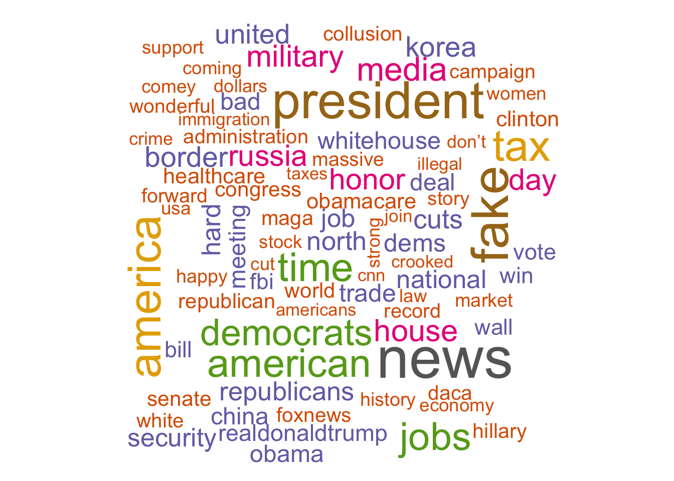
The Term Frequency - Inverse Document Frequency is a commonly used
metric for text data where the frequency of terms is considered
alongside the uniqueness of terms to produce a measurement of word
importance. The tf–idf value increases proportionally to the number of
times a word appears in the document and is offset by the number of
documents in the corpus that contain the word, which helps to adjust for
the fact that some words appear more frequently in general. Use the
bind_tf_idf() function for this calculation.
trump_tfidf <- tidy_trumps %>%
  count(word, created_at) %>%
  bind_tf_idf(word, created_at, n) %>%
  arrange(desc(tf_idf))

head(trump_tfidf)
## # A tibble: 6 × 6
## word created_at n tf idf tf_idf
## <chr> <dttm> <int> <dbl> <dbl> <dbl>
## 1 brazoriacounty 2017-08-29 16:06:57 1 1 8.07 8.07
## 2 congressionalbaseballgame 2017-06-15 23:49:24 1 1 8.07 8.07
## 3 luisriveramarin 2017-10-31 15:48:22 1 1 8.07 8.07
## 4 nicole 2017-08-05 23:01:05 1 1 8.07 8.07
## 5 senatordole 2017-07-09 00:29:21 1 1 8.07 8.07
## 6 usembassyjerusalem 2018-05-14 15:16:38 1 1 8.07 8.07Let’s visualize some tweets over time using the tfidf scores. First, let’s convert the created_at column to a Date class using the POSIXct class converter. This helps with time-based analysis as date becomes a more manipulable data type.
trump_tfidf$created_at <- as.Date(as.POSIXct(trump_tfidf$created_at))The following code will produce seven plots that include counts of the top ten tokens used on a given day in terms of tfidf. See the comments for how to read each line of code.
trump_tfidf %>% #update the object trump_tfidf where
  filter(created_at >= as.Date("2018-05-12")) %>% #the date must be greater than or equal to May 12th, 2018
  group_by(created_at) %>% #and the data set is grouped by the same column
  top_n(10, tf_idf) %>% #with only the top 10 tfidf scores
  ungroup() %>% #we then ungroup the date
  mutate(word = reorder(word, tf_idf)) %>% #so that words can be ordered by tfidf
  ggplot(aes(word, tf_idf, fill = created_at)) + #and plotted with words on the x axis and tf_idf on the y axis
  geom_col(show.legend = FALSE) + #and legends removed
  facet_wrap(~created_at, scales = "free") + #with multiple plots free to expand to the maximum in either dimension
coord_flip() #with x and y coordinates then flipped so that text data are more readable. 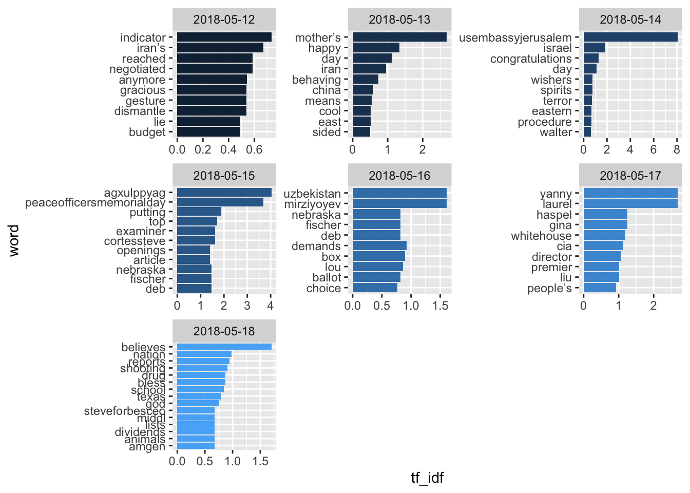
8.4 Sentiment Analysis
Sentiment analysis is the process of computationally identifying and
categorizing opinions expressed in a piece of text. The sentimentr
package makes ‘opinion mining’ easy. For instance, the sentiment()
function was deployed below on four separate strings, one including two
sentences. Compare the output of these four chunks.
sentiment('Sentiment analysis is super fun.')## element_id sentence_id word_count sentiment
## 1: 1 1 5 0.6708204sentiment('I hate sentiment analysis.')## element_id sentence_id word_count sentiment
## 1: 1 1 4 -0.375sentiment('Sentiment analysis is okay.')## element_id sentence_id word_count sentiment
## 1: 1 1 4 0sentiment('Sentiment analysis is super boring. I do love working in R though.')## element_id sentence_id word_count sentiment
## 1: 1 1 5 -0.1118034
## 2: 1 2 7 0.3779645The sentiment column reflects a number from -1 to +1 that is associated
with the negative or positive valence of a particular comment. This
works as the sentimentR package includes labelled lists of words which
are then calculated alongside each other as part of word patterns.
Therefore, the package is able to distinguish neutral, positive, and
negatively phrased strings.
8.4.1 Case Study Two
For our second case study we are going to be using the harrypotter dataset, which includes the full text from the entire Harry Potter series. For the source code see https://github.com/bradleyboehmke/harrypotter.
First, set books as an array where each value in the array is a chapter.
Each book is an array in which each value in the array is a chapter. In
the code below, unnest_tokens() is deployed on each chapter at the
word level for subsequent analysis.
books <- list(philosophers_stone, chamber_of_secrets, prisoner_of_azkaban,
              goblet_of_fire, order_of_the_phoenix, half_blood_prince,
              deathly_hallows)

titles <- c("Philosopher's Stone", "Chamber of Secrets", "Prisoner of Azkaban",
            "Goblet of Fire", "Order of the Phoenix", "Half-Blood Prince",
            "Deathly Hallows")

series <- tibble()
for(i in seq_along(titles)) {

  temp <- tibble(chapter = seq_along(books[[i]]), text = books[[i]]) %>%
    unnest_tokens(word, text) %>%
    mutate(book = titles[i]) %>%
    select(book, everything())

  series <- rbind(series, temp)
}
Set a factor to keep books ordered by publication date and chapter.
series$book <- factor(series$book, levels = rev(titles))
series
## # A tibble: 1,089,386 × 3
## book chapter word
## <fct> <int> <chr>
## 1 Philosopher's Stone 1 the
## 2 Philosopher's Stone 1 boy
## 3 Philosopher's Stone 1 who
## 4 Philosopher's Stone 1 lived
## 5 Philosopher's Stone 1 mr
## 6 Philosopher's Stone 1 and
## 7 Philosopher's Stone 1 mrs
## 8 Philosopher's Stone 1 dursley
## 9 Philosopher's Stone 1 of
## 10 Philosopher's Stone 1 number
## # … with 1,089,376 more rowshead(series)## # A tibble: 6 × 3
## book chapter word
## <fct> <int> <chr>
## 1 Philosopher's Stone 1 the
## 2 Philosopher's Stone 1 boy
## 3 Philosopher's Stone 1 who
## 4 Philosopher's Stone 1 lived
## 5 Philosopher's Stone 1 mr
## 6 Philosopher's Stone 1 andThis code will produce the most frequently appearing words in the series.
head(series %>% count(word, sort = TRUE))## # A tibble: 6 × 2
## word n
## <chr> <int>
## 1 the 51593
## 2 and 27430
## 3 to 26985
## 4 of 21802
## 5 a 20966
## 6 he 20322Let’s see how removing stop words impacts that list and display the results with a wordcloud.
series %>%
  anti_join(stop_words) %>%
  count(word, sort = TRUE) %>%
  with(wordcloud(word, n, max.words = 50))
## Joining, by = "word"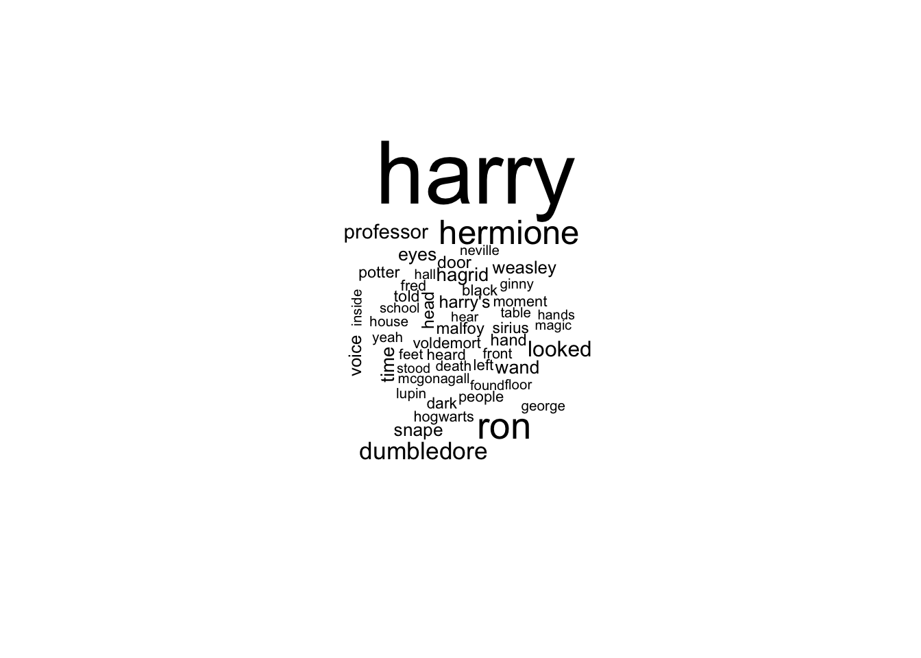
As previously mentioned, there are datasets which are labelled for sentiment. Below we right join the list of sentiment tokens to our harrypotter corpus word list.
series %>%
  right_join(get_sentiments("nrc")) %>% # nrc is the name of data set
  filter(!is.na(sentiment)) %>%  # filter
  count(sentiment, sort = TRUE)
## Joining, by = "word"## # A tibble: 10 × 2
## sentiment n
## <chr> <int>
## 1 negative 55093
## 2 positive 37758
## 3 sadness 34878
## 4 anger 32743
## 5 trust 23154
## 6 fear 21536
## 7 anticipation 20625
## 8 joy 13800
## 9 disgust 12861
## 10 surprise 12817nrc filters for positive/negative valence, and has predetermined
emotional classifiers built in, while bing only uses positive/negative
valence.
series %>%
  right_join(get_sentiments("bing")) %>%
  filter(!is.na(sentiment)) %>%
  count(sentiment, sort = TRUE)
## Joining, by = "word"## # A tibble: 2 × 2
## sentiment n
## <chr> <int>
## 1 negative 39502
## 2 positive 29065This example brings in the bing word list which is joined to the words
in the harrypotter corpus alongside the sentiment scores, and then plots
the top positive and negative words in the same wordcloud.
series %>%
  inner_join(get_sentiments("bing")) %>%
  count(word, sentiment, sort = TRUE) %>%
  acast(word ~ sentiment, value.var = "n", fill = 0) %>%
  comparison.cloud(colors = c("#F8766D", "#00BFC4"),
                   max.words = 50)
## Joining, by = "word"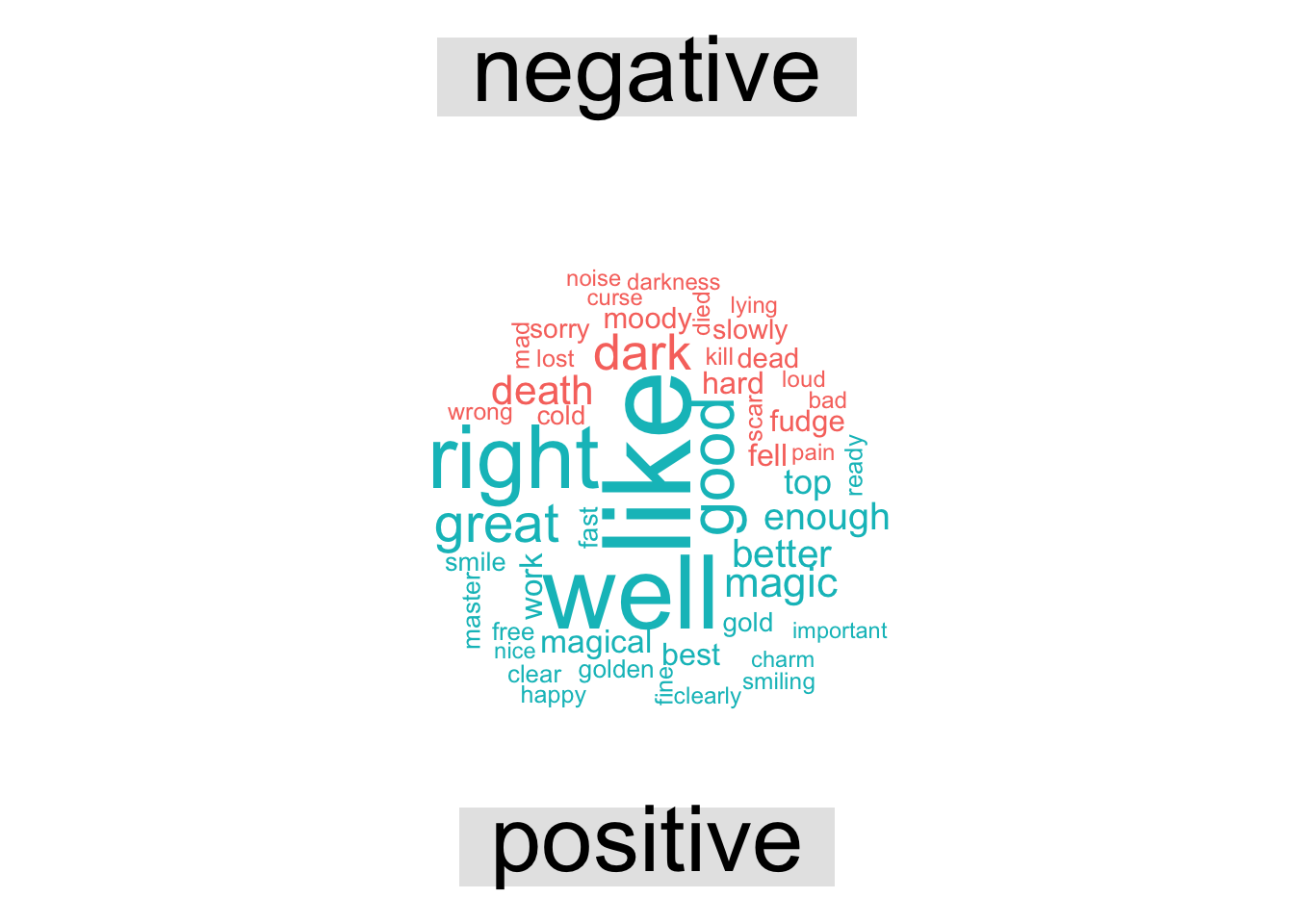
Did you notice that example left stopwords in? Let’s see how it looks
with a stopword anti_join().
series %>%
  anti_join(stop_words) %>%
  inner_join(get_sentiments("bing")) %>%
  count(word, sentiment, sort = TRUE) %>%
  acast(word ~ sentiment, value.var = "n", fill = 0) %>%
  comparison.cloud(colors = c("#F8766D", "#00BFC4"),
                   max.words = 50)
## Joining, by = "word"
## Joining, by = "word"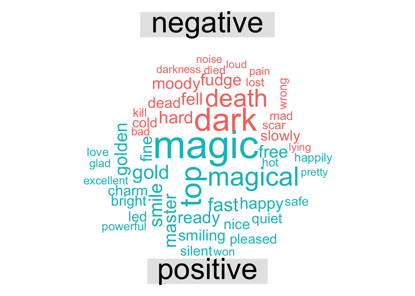
In this next bit of code, we are going to group by words in each book, bring in bing sentiments, count words and sentiment before plotting a geom including the sentiment of words used in each book.
series %>%
  group_by(book) %>%
  mutate(word_count = 1:n(),
         index = word_count %/% 500 + 1) %>%
  inner_join(get_sentiments("bing")) %>%
  count(book, index = index , sentiment) %>%
  spread(sentiment, n, fill = 0) %>%
  mutate(sentiment = positive - negative,
         book = factor(book, levels = titles)) %>%
  ggplot(aes(index, sentiment, fill = book)) +
  geom_bar(alpha = 0.5, stat = "identity", show.legend = FALSE) +
  facet_wrap(~ book, ncol = 2, scales = "free_x")
## Joining, by = "word"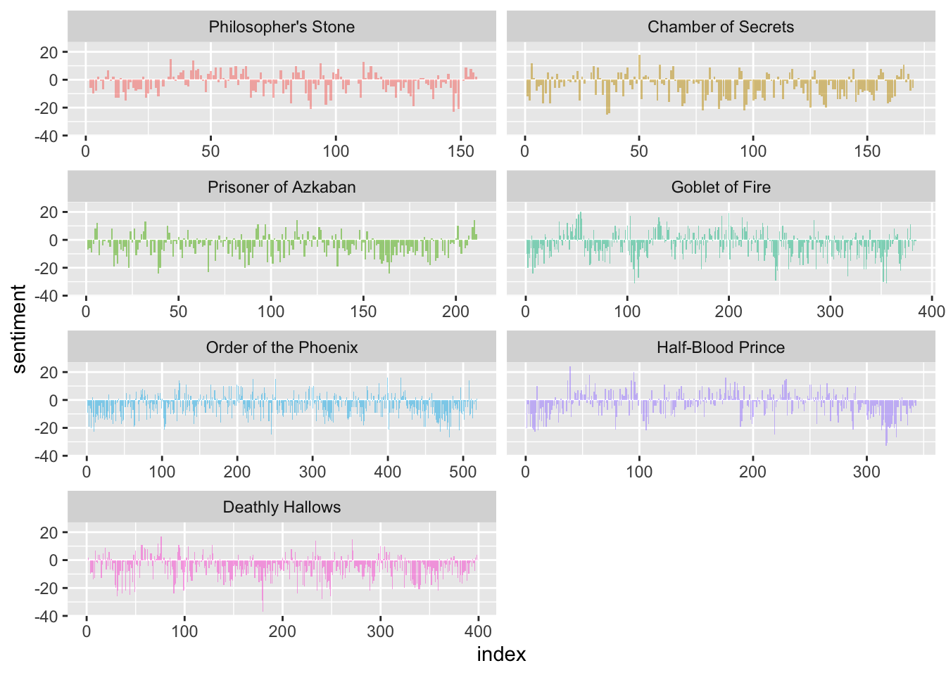
To investigate bigrams, use the unnest() function where token = ngrams, and n = 2, and mutate our dataframe accordingly. We then need to order the books appropriately by setting them as a factor once more.
series <- tibble()
for(i in seq_along(titles)) {

  temp <- tibble(chapter = seq_along(books[[i]]),
                  text = books[[i]]) %>%
    unnest_tokens(bigram, text, token = "ngrams", n = 2) %>%
    mutate(book = titles[i]) %>%
    select(book, everything())

  series <- rbind(series, temp)
}
series$book <- factor(series$book, levels = rev(titles))
Much like word frequencies, this code will count the top bigrams in the dataset.
series %>%
  count(bigram, sort = TRUE)
## # A tibble: 340,021 × 2
## bigram n
## <chr> <int>
## 1 of the 4895
## 2 in the 3571
## 3 said harry 2626
## 4 he was 2490
## 5 at the 2435
## 6 to the 2386
## 7 on the 2359
## 8 he had 2138
## 9 it was 2123
## 10 out of 1911
## # … with 340,011 more rowsBigrams, like words, can be filtered and cleaned to remove stop words and other noise.
bigrams_separated <- series %>%
  separate(bigram, c("word1", "word2"), sep = " ")
bigrams_filtered <- bigrams_separated %>%
  filter(!word1 %in% stop_words$word) %>%
  filter(!word2 %in% stop_words$word)

head(bigrams_separated)
## # A tibble: 6 × 4
## book chapter word1 word2
## <fct> <int> <chr> <chr>
## 1 Philosopher's Stone 1 the boy
## 2 Philosopher's Stone 1 boy who
## 3 Philosopher's Stone 1 who lived
## 4 Philosopher's Stone 1 lived mr
## 5 Philosopher's Stone 1 mr and
## 6 Philosopher's Stone 1 and mrshead(bigrams_filtered)## # A tibble: 6 × 4
## book chapter word1 word2
## <fct> <int> <chr> <chr>
## 1 Philosopher's Stone 1 privet drive
## 2 Philosopher's Stone 1 perfectly normal
## 3 Philosopher's Stone 1 firm called
## 4 Philosopher's Stone 1 called grunnings
## 5 Philosopher's Stone 1 usual amount
## 6 Philosopher's Stone 1 time craningHere are our updated bigram counts with clean data.
bigrams_united <- bigrams_filtered %>%
  unite(bigram, word1, word2, sep = " ")
head(bigrams_united %>%
    count(bigram, sort = TRUE))
## # A tibble: 6 × 2
## bigram n
## <chr> <int>
## 1 professor mcgonagall 578
## 2 uncle vernon 386
## 3 harry potter 349
## 4 death eaters 346
## 5 harry looked 316
## 6 harry ron 302bind_tf_idf() works for bigrams too.
bigram_tf_idf <- bigrams_united %>%
  count(book, bigram) %>%
  bind_tf_idf(bigram, book, n) %>%
  arrange(desc(tf_idf))
head(bigram_tf_idf)
## # A tibble: 6 × 6
## book bigram n tf idf tf_idf
## <fct> <chr> <int> <dbl> <dbl> <dbl>
## 1 Order of the Phoenix professor umbridge 173 0.00533 1.25 0.00667
## 2 Prisoner of Azkaban professor lupin 107 0.00738 0.847 0.00625
## 3 Deathly Hallows elder wand 58 0.00243 1.95 0.00473
## 4 Goblet of Fire ludo bagman 49 0.00201 1.95 0.00391
## 5 Prisoner of Azkaban aunt marge 42 0.00290 1.25 0.00363
## 6 Deathly Hallows death eaters 139 0.00582 0.560 0.00326Use this code to display the bigrams with the highest TF-IDF scores across the series.
plot_potter<- bigram_tf_idf %>%
  arrange(desc(tf_idf)) %>%
  mutate(bigram = factor(bigram, levels = rev(unique(bigram))))

plot_potter %>%
  top_n(20) %>%
  ggplot(aes(bigram, tf_idf, fill = book)) +
  geom_col() +
  labs(x = NULL, y = "tf-idf") +
  coord_flip()
## Selecting by tf_idf
We may be overestimating the negative sentiment in the data set due to negatives. Deal with negatives by filtering and removing words that are associated with ‘not.’
bigrams_separated %>%
  filter(word1 == "not") %>%
  count(word1, word2, sort = TRUE)
## # A tibble: 1,085 × 3
## word1 word2 n
## <chr> <chr> <int>
## 1 not to 383
## 2 not be 157
## 3 not a 131
## 4 not have 116
## 5 not the 103
## 6 not know 98
## 7 not going 92
## 8 not want 81
## 9 not said 76
## 10 not been 75
## # … with 1,075 more rowsbigrams_separated <- bigrams_separated %>%
filter(word1 == "not") %>%
filter(!word2 %in% stop_words$word)%>%
count(word1, word2, sort = TRUE)
head(bigrams_separated)## # A tibble: 6 × 3
## word1 word2 n
## <chr> <chr> <int>
## 1 not answer 41
## 2 not speak 41
## 3 not understand 35
## 4 not harry 32
## 5 not supposed 25
## 6 not dare 248.5 Networks with Hamilton Lyrics
See this code for an application of network analysis on the corpus from Hamilton. This code was taken from this tutorial: https://cfss.uchicago.edu/notes/hamilton/
library(widyr)
library(ggraph)
library(tidyverse)
library(tidytext)
library(ggtext)
library(here)
## here() starts at /Users/jbh6331/Desktop/R/IDSRset.seed(123)
theme_set(theme_minimal())
hamilton <- read_csv(file = here("hamilton.csv")) %>%
mutate(song_name = parse_factor(song_name))## Rows: 3532 Columns: 5## ── Column specification ────────────────────────────────────────────────────────
## Delimiter: ","
## chr (3): song_name, line, speaker
## dbl (2): song_number, line_num
##
## ℹ Use `spec()` to retrieve the full column specification for this data.
## ℹ Specify the column types or set `show_col_types = FALSE` to quiet this message.# calculate all pairs of words in the musical
hamilton_pair <- hamilton %>%
unnest_tokens(output = word, input = line, token = "ngrams", n = 2) %>%
separate(col = word, into = c("word1", "word2"), sep = " ") %>%
filter(!word1 %in% get_stopwords(source = "smart")$word,
!word2 %in% get_stopwords(source = "smart")$word) %>%
drop_na(word1, word2) %>%
count(word1, word2, sort = TRUE)
# filter for only relatively common combinations
bigram_graph <- hamilton_pair %>%
filter(n > 3) %>%
igraph::graph_from_data_frame()
# draw a network graph
set.seed(1776) # New York City
ggraph(bigram_graph, layout = "fr") +
geom_edge_link(aes(edge_alpha = n, edge_width = n), show.legend = FALSE, alpha = .5) +
geom_node_point(color = "#0052A5", size = 3, alpha = .5) +
geom_node_text(aes(label = name), vjust = 1.5) +
ggtitle("Word Network in Lin-Manuel Miranda's *Hamilton*") +
theme_void() +
theme(plot.title = element_markdown())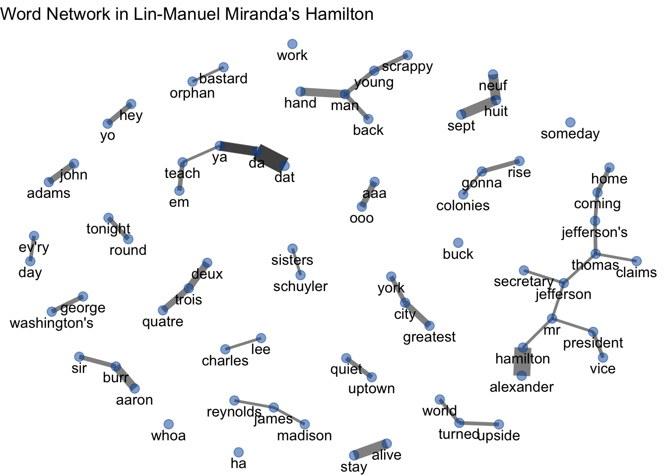
8.6 Topic Modeling
A traditional content analysis might utilize keyword counting, thematic coding, and other human-driven data categorization to contextualize text data. Instead, we can use a Latent Dirichlet Allocation (LDA) process on the corpora, a machine learning technique that emerged as part of developments in the artificial intelligence field (Gropp & Herzog, 2016). In essence, LDA identifies latent constructs within a corpus through the identification of co-occurring word patterns and semantically similar clustered word combinations. These methods have increased in popularity across the social sciences in the past decade, as robust algorithms allow researchers to investigate the inner workings of text-based data while limiting their bias. LDA algorithms examine entire corpora in minutes, illuminating “statistical regularities in word co-occurrence that often correspond to recognizable themes, events, or discourses” (Baumer, et al., 2017, p. 1398). The output of these algorithms is referred to as a topic model.
Topic model data typically includes a numerical set of topic labels (e.g. topic 0, topic 1, topic 2), a set of keywords that are associated with each topic, and a list of representative sentences for each topic. The algorithm assigns these sentences to each topic based on the prevalence of the topic keywords within the text. In the LDA process, unique keywords are assigned numerical values (e.g. Young = 0, People’s = 1, Concerts = 2, and so on). Using these values, the representativeness of each sentence is measured with a logistic distribution and is then assigned a document-topic probability score between 0 and 1. The higher the score, the better the probability that the topic of the sentence provides represents a larger subset of a corpus.
To get started, let’s convert the tidy_ham word column to a corpus from
the tm library.
tidy_ham <- hamilton %>%
  select(song_name, line) %>%
  unnest_tokens("word", line) %>%
  anti_join(stop_words) #%>%
## Joining, by = "word" #mutate_at("word", funs(wordStem((.), language="en")))
ham_corpus <-iconv(tidy_ham$word)
corpus <- Corpus(VectorSource(ham_corpus))
corpus## <<SimpleCorpus>>
## Metadata: corpus specific: 1, document level (indexed): 0
## Content: documents: 7338We now transform all upper case to lower case, as well as remove punctuation, stop words, numbers, and whitespace.
corpus <- tm_map(corpus, content_transformer(tolower)) ## Warning in tm_map.SimpleCorpus(corpus, content_transformer(tolower)):
## transformation drops documentscorpus <- tm_map(corpus, removePunctuation) ## Warning in tm_map.SimpleCorpus(corpus, removePunctuation): transformation drops
## documentscorpus <- tm_map(corpus,removeWords,stopwords("english"))## Warning in tm_map.SimpleCorpus(corpus, removeWords, stopwords("english")):
## transformation drops documentscorpus <- tm_map(corpus, removeNumbers)## Warning in tm_map.SimpleCorpus(corpus, removeNumbers): transformation drops
## documentscorpus <- tm_map(corpus, stripWhitespace) ## Warning in tm_map.SimpleCorpus(corpus, stripWhitespace): transformation drops
## documentscorpus## <<SimpleCorpus>>
## Metadata: corpus specific: 1, document level (indexed): 0
## Content: documents: 7338The document term matrix (dtm) is our new dataframe. Topic model packages interact with dtm’s to construct possible models
dtm <- DocumentTermMatrix(corpus)
dtm
## <<DocumentTermMatrix (documents: 7338, terms: 2447)>>
## Non-/sparse entries: 7103/17948983
## Sparsity : 100%
## Maximal term length: 18
## Weighting : term frequency (tf)More cleaning. This code will create an index for each token.
rowTotals <- apply(dtm,1,sum) #running this line takes time
empty.rows <- dtm[rowTotals==0,]$dimnames[1][[1]]
corpus <- corpus[-as.numeric(empty.rows)]
dtm <- DocumentTermMatrix(corpus)
dtm
## <<DocumentTermMatrix (documents: 7103, terms: 2447)>>
## Non-/sparse entries: 7103/17373938
## Sparsity : 100%
## Maximal term length: 18
## Weighting : term frequency (tf)Use the inspect() function to see how the dtm counts text by index.
inspect(dtm[1:5, 1:5])## <<DocumentTermMatrix (documents: 5, terms: 5)>>
## Non-/sparse entries: 5/20
## Sparsity : 80%
## Maximal term length: 8
## Weighting : term frequency (tf)
## Sample :
## Terms
## Docs bastard orphan scotsman son whore
## 1 1 0 0 0 0
## 2 0 1 0 0 0
## 3 0 0 0 1 0
## 4 0 0 0 0 1
## 5 0 0 1 0 0Sum and sort these word counts.
dtm.mx <- as.matrix(dtm)
frequency <- colSums(dtm.mx)
frequency <- sort(frequency, decreasing=TRUE)
frequency[1:25]
## wait time hamilton hey burr shot sir alexander
## 81 79 77 73 65 58 56 51
## whoa president gonna rise world story satisfied alive
## 42 39 38 37 36 35 35 34
## york home helpless angelica jefferson fight dat eyes
## 33 32 32 31 30 29 27 27
## write
## 26Topic models must have the number of potential topics specified. There are many ways to go about this, though some researchers depend on trial and error in an iterative process while they check the appropriateness of model output. Four alternative automated approaches are included in the plot below. These models predict the latent distribution of document topic probabilities to produce the best model. Read this output by seeing where the models intersect on each graph.
result <- FindTopicsNumber(
  dtm,
  topics = seq(from = 2, to = 50, by = 1),
  metrics = c("Griffiths2004", "CaoJuan2009", "Arun2010", "Deveaud2014"),
  method = "Gibbs",
  control = list(seed = 77),
  mc.cores = 2L,
  verbose = TRUE
)
## fit models... done.
## calculate metrics:
## Griffiths2004... done.
## CaoJuan2009... done.
## Arun2010... done.
## Deveaud2014... done.FindTopicsNumber_plot(result)## Warning: `guides(<scale> = FALSE)` is deprecated. Please use `guides(<scale> =
## "none")` instead.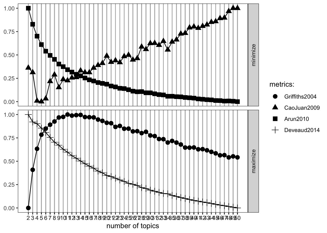
For a deep dive on each of the parameters in the topic models package, see the documentation here: https://cran.r-project.org/web/packages/topicmodels/topicmodels.pdf
For now, all we should focus on is k, which represents the number of topics you are feeding into your model. Based on the previous graph, we should let the model assign 9 topics based on a general interpretation of the previous plot.
#set model parameters
burnin <- 4000
iter <- 2000
thin <- 500
seed <-list(2003,5,63,100001,765)
nstart <- 5
best <- TRUE
k <- 9
Convert your LDA model to be readable by the LDAvis package.
ldaOut <-LDA(dtm, k, method="Gibbs", control=list(nstart=nstart, seed = seed, best=best, burnin = burnin, iter = iter, thin=thin))
ldaOut.topics <- as.matrix(topics(ldaOut))
See the top six terms in each topic.
ldaOut.terms <- as.matrix(terms(ldaOut, 6))
ldaOut.terms
## Topic 1 Topic 2 Topic 3 Topic 4 Topic 5 Topic 6
## [1,] "sir" "hey" "shot" "wait" "hey" "time"
## [2,] "york" "president" "gonna" "gotta" "alive" "son"
## [3,] "helpless" "whoa" "hamilton" "life" "alexander" "war"
## [4,] "wrote" "story" "rise" "ooh" "choose" "gon"
## [5,] "happened" "wanna" "city" "time" "sister" "mind"
## [6,] "love" "day" "father" "boom" "goodbye" "history"
## Topic 7 Topic 8 Topic 9
## [1,] "hamilton" "home" "burr"
## [2,] "world" "jefferson" "time"
## [3,] "fight" "alexander" "angelica"
## [4,] "throwing" "eyes" "eliza"
## [5,] "lafayette" "satisfied" "hamilton"
## [6,] "evry" "revolution" "stand"This code prepares your LDA visualization.
topicmodels2LDAvis <- function(x, ...){
  post <- topicmodels::posterior(x)
  if (ncol(post[["topics"]]) < 3) stop("The model must contain > 2 topics")
  mat <- x@wordassignments
  LDAvis::createJSON(
    phi = post[["terms"]],
    theta = post[["topics"]],
    vocab = colnames(post[["terms"]]),
    doc.length = slam::row_sums(mat, na.rm = TRUE),
    term.frequency = slam::col_sums(mat, na.rm = TRUE)
  )
}
Finally, display your LDA using LDAvis.
serVis(topicmodels2LDAvis(ldaOut))8.6.1 A Note on Word Embeddings
Word embeddings allow researchers to investigate semantically similar words that do not have the same stem (e.g. anxious and confused). The text below is from a tutorial (linked below) that visualizes text data in the word embedding space along different dimensions such as rating scores. This allows for more quantitative analysis of text data. Link to article here:
install.packages('text')
library(text)
# Use data (DP_projections_HILS_SWLS_100) that have been pre-processed with the textProjectionData function; the preprocessed test-data included in the package is called: DP_projections_HILS_SWLS_100
plot_projection <- textProjectionPlot(
  word_data = DP_projections_HILS_SWLS_100,
  y_axes = TRUE,
  title_top = " Supervised Bicentroid Projection of Harmony in life words",
  x_axes_label = "Low vs. High HILS score",
  y_axes_label = "Low vs. High SWLS score",
  position_jitter_hight = 0.5,
  position_jitter_width = 0.8
)
plot_projection
#> $final_plot
8.7 Review
In this chapter we introduced text analysis concepts and methods. To make sure you understand this material, there is a practice assessment to go along with this chapter at <https://jayholster.shinyapps.io/Text>AnalysisinRAssessment.
8.8 References
Csardi, G., Nepusz, T. (2006). “The igraph software package for complex network research.” InterJournal, Complex Systems, 1695. https://igraph.org.
Grun, B., Hornik, K., Blei, D. M., Lafferty, J. D., Phan, X. H., Matsumoto, M., Nishimura, T., & Cobus, S. (2021). Topic models. https://cran.r-project.org/web/packages/topicmodels/index.html
Fellows, I. (2018). wordcloud. https://cran.r-project.org/web/packages/wordcloud/index.html
Feinerer, I., Hornik, K., & Meyer, D. (2008). “Text Mining Infrastructure in R.” Journal of Statistical Software, 25(5), 1–54. https://www.jstatsoft.org/v25/i05/.
Gogolewski, M., Tarantus, B., & others (2021). Stringi. https://cran.r-project.org/web/packages/stringi/index.html
Grolemund, G., &Wickham, H. (2011). Dates and times made easy with lubridate. Journal of Statistical Software, 40(3), 1–25. https://www.jstatsoft.org/v40/i03/.
Nikita, M., & Chaney, N. (2020). Ldatuning. https://cran.r-project.org/web/packages/ldatuning/index.html
Hvitfeldt, E., & Silge, J. (2022). textdata. https://cran.r-project.org/web/packages/textdata/index.html
Porter, M., Boulton, R., & Bouchet-Valat, M. (2013). SnowballC. https://cran.r-project.org/web/packages/SnowballC/index.html
Rinker, T.W. (2021). sentimentr: Calculate Text Polarity Sentiment. version 2.9.0, <https://github.com/trinker/sentimentr>.
Robinson, D. (2021). gutenbergr. https://cran.r-project.org/web/packages/gutenbergr/index.html
Sievert, C., & Shirley, K. (2015). LDAvis. https://cran.r-project.org/web/packages/LDAvis/index.html
Silge, J., Robinson, D. (2016). tidytext: Text mining and analysis using tidy data principles in R.” JOSS, 1(3). https://[doi:10.21105/joss.00037](https://%5Bdoi:10.21105/joss.00037){.uri}.
Tyner, S., Briatte, F., & Hofmann, H. (2017). Network Visualization
with ggplot2, The R Journal
9(1): 27–59. https://briatte.github.io/ggnetwork/
Wickham, H. (2022). reshape. https://cran.r-project.org/web/packages/reshape/index.html
Wickham, H., Averick, M., Bryan, J., Chang, W., McGowan, L.D., François, R., Grolemund, G., Hayes, A., Henry, L., Hester, J., Kuhn, M., Pedersen, T.L., Miller, E., Bache, S.M., Müller, K., Ooms, J., Robinson, D., Seidel, D.P., Spinu, V., Takahashi, K., Vaughan, D., Wilke, C., Woo, K., & Yutani, H. (2019). Welcome to the tidyverse. Journal of Open Source Software, 4(43), 1686. https://doi.org/10.21105/joss.01686.
Xie, Y., Sievert, C., Anderson, J., Vaidyanathan, R., & Lesur, R. (2021). servr. https://cran.r-project.org/web/packages/servr/index.html
8.8.1 R Short Course Series
Video lectures of each guidebook chapter can be found at https://osf.io/6jb9t/. For this chapter, find the follow the folder path Text Analysis in R -> AY 2021-2022 Spring and access the video files, r markdown documents, and other materials for each short course.
8.8.2 Acknowledgements
This guidebook was created with support from the Center for Research Data and Digital Scholarship and the Laboratory for Interdisciplinary Statistical Analaysis at the University of Colorado Boulder, as well as the U.S. Agency for International Development under cooperative agreement #7200AA18CA00022. Individuals who contributed to materials related to this project include Jacob Holster, Eric Vance, Michael Ramsey, Nicholas Varberg, and Nickoal Eichmann-Kalwara.