Introduction to R for Data Science: A LISA 2020 Guidebook
2022-07-10
Chapter 1 R Foundations
Data science is emerging as a vital skill for researchers, analysts, librarians, and others who deal with data in their personal and professional work. In essence, data science is the application of the scientific method to data for the purpose of understanding the world we live in. More specifically, data science tasks emerge from an interdisciplinary amalgam of statistical analysis, computer science, and social science research conventions. Although other programming languages such as python exceed R in general popularity, R remains as one of the most popular programming languages for data scientists and researchers due to a focus on statistical programming. As such, R and RStudio are invaluable tools to the data scientist, statistician, researcher, and many others.
This guidebook aims to provide readers an opportunity to make a start towards learning R for a variety of data science tasks, include (a) data cleaning and preparation, (b) statistical analysis, (c) data visualization, (d) natural language processing, (e) network analysis, and (f) Structural Equation Modeling to name a few. In Chapters 1 and 2 we invite readers to install R and RStudio and to start manipulating data for analysis. Chapter 3 and Chapter 4 include introductory exercises to teach data visualization and statistical analysis in R. In Chapter 5 and beyond, you will explore basic analytic concepts (e.g., correlation and regression) and more advanced approaches to data modeling through the lenses of Structural Equation Modeling, Network Analysis, and Text Analysis.
By the end of this guidebook, among several other skills, you will be able to use R to visualize distributions of data across categorical groups, such as in the example below:
library(ggstatsplot)
library(tidyverse)
data <- read_csv('musicclassintentions.csv')

ggbetweenstats(
  data = data,
  x = Level,
  y = intentions,
  title = "Distribution of Intentions to Sign Up for Music Across Grade Level"
)
Calculate correlation coefficients, and visualize relationships between your data:
library(psych)
library(tidyverse)

variablelist <- data %>% select(intentions, values, needs, parentsupport, SESComp)
psych::pairs.panels(variablelist,
             method = "pearson", # correlation method
             hist.col = "#00AFBB",
             density = TRUE,  # show density plots
             ellipses = TRUE,
             lm = TRUE# show correlation ellipses
             )
Fit General Linear Models (GLM) and produce publishable tables:
library(tidyverse)
library(knitr)
library(broom)

tidy(lm(intentions ~ SESComp + parentsupport + needs + values, data=data)) %>%
  kable(caption = "Estimates for Variation in Music Elective Intentions.",
    col.names = c("Predictor", "B", "SE", "t", "p"),
digits = c(0, 2, 3, 2, 3))| Predictor | B | SE | t | p |
|---|---|---|---|---|
| (Intercept) | -5.42 | 6.261 | -0.87 | 0.394 |
| SESComp | 3.87 | 1.639 | 2.36 | 0.025 |
| parentsupport | 0.52 | 0.306 | 1.69 | 0.101 |
| needs | -0.28 | 0.115 | -2.40 | 0.023 |
| values | 0.28 | 0.072 | 3.90 | 0.001 |
Fit, interpret, and visualize Structural Equation Models (SEM):
library(lavaan)
library(semPlot)

model <- '
  # regressions
    needs ~ parentsupport
    values ~ needs + parentsupport + peersupport
    intentions ~ values + needs + SESComp'

fit <- sem(model, data=data)

semPaths(fit, what = "path", whatLabels = "std", style = "lisrel", edge.label.cex = .9, rotation = 2, curve = 3, layoutSplit = FALSE, normalize = FALSE, height = 9, width = 6.5, residScale = 10)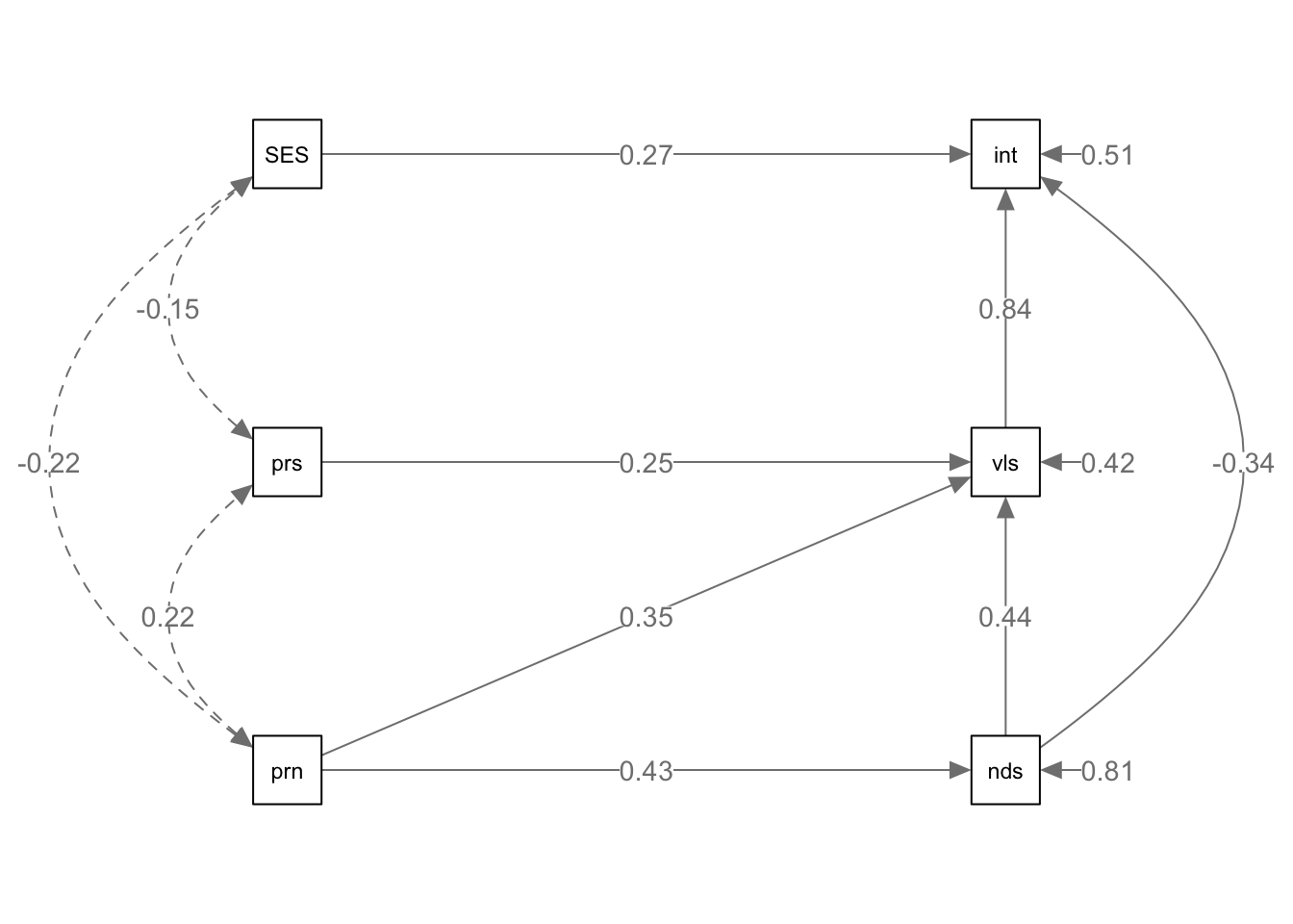
As well as clean text data and analyze large corpora through the lenses of machine learning concepts such as sentiment analysis and topic modeling:
library(sentimentr)
sentiment('Sentiment analysis is super fun. I hate sentiment analysis. Sentiment analysis is okay')
## element_id sentence_id word_count sentiment
## 1: 1 1 5 0.6708204
## 2: 1 2 4 -0.3750000
## 3: 1 3 4 0.0000000Each concept is presented with unique datasets, including qualitative data from Harry Potter, Hamilton, and Donald Trump Tweets, and quantitative data from baseR datasets such as mtcars, elective intentions data for middle school students, and other real world data.
Additionally, there will be an informal assessment tied to each chapter so you can test and apply your skills as you move through the book.
1.1 Getting Started with R and RStudio
This chapter contains an introduction to the installation of R, how to install packages, and an introduction to object-based coding concepts. If you are having trouble downloading R and installing your first packages, please view the optional check in assessment at https://jayholster.shinyapps.io/RLevel0Assessment/ Take a few minutes to download and install both R and RStudio. They are both free and easy to download.
Download R from <https://cran.r-project.org/> Choose your operating system (Windows, MacOS, or Linux) and download as you would any other program.
Download the free version of RStudio for your OS from <https://www.rstudio.com/products/rstudio/download/> Follow prompts to install.
According to Rstudio’s documentation, <https://cran.r-project.org/doc/contrib/Paradis-rdebuts_en.pdf>): “when R is running, variables, data, functions, results, etc, are stored in the active memory of the computer in the form of objects which have a name. The user can do actions on these objects with operators (arithmetic, logical,comparison, . . .) and functions (which are themselves objects).” We will explore the concept and capabilities of the obect throughout this text.
1.1.1 The Integrated Development Environment
Where R is a programming language, RStudio is an integrated development environment (IDE) which enables users to efficiently access and view most facets of the program in a four pane environment. These include the source, console, environment and history, as well as the files, plots, packages and help. The console is in the lower-left corner, and this is where commands are entered and output is printed. The source pane is in the upper-left corner, and is a built in text editor. While the console is where commands are entered, the source pane includes executable code which communicates with the console. The environment tab, in the upper-right corner displays an list of loaded R objects. The history tab tracks the user’s keystrokes entered into the console. Tabs to view plots, packages, help, and output viewer tabs are in the lower-right corner.
Where SPSS and other menu based analytic software are limited by user input and installed software features, R operates as a mediator between user inputs and open source developments from our colleagues all over the world. This affords R users a certain flexibility. However, it takes a few extra steps to appropriately launch projects. Regardless of your needs with R, you will likely interact with the following elements of document set up.
1.1.2 Learning to Read Code
“Numquam ponenda est pluralitas sine necessitate. Plurality is never to be posited without necessity.”
William of Occam, circa 1495
The most formidable challenge many new R users face is learning to code. While coding can seem daunting at first, it is important to remember that all coding tasks simply involve solutions to problems the user identifies. No matter how difficult the problem, there are always a lot of solutions to each problems, and someone else has always encountered the solution, and likely has posted it to a forum. Occams Razor (i.e., the solution with the least amount of assumptions is the best) helps you identify the problems to solve as you interact with code. For new users, your breakthrough moment where you start to feel like a programmer might come from a well-worded google search and a focused effort to solve an issue with the R programming language. It is, indeed, a language, so half of the battle is learning to read code in a manner that is meaningful to you. Throughout this guidebook, you will be provided with tutorials and suggestions for reading the code you interact with. In this first chapter, you will start to encounter objects, functions, arguments, and operators. It is important to develop code reading fluency. As such, I encourage readers to speak code out loud to themselves as they interact with this guidebook.
1.1.3 Practices in Reproducibility
It is important—whether you are working alone or with others—to adopt a collaboration mindset. This value is clearly important when working with other statistical collaborators or with domain experts who do not have experience in R. Even experienced users might become confused when examining a peer’s code. The same effect may occur if you return to a project after many months, and find yourself lost in your own code. As such, I recommend utilizing R markdown files (File -> New File -> R Markdown)and comments # to provide notes to yourself and others who might interact with your code. For instance, this is an R Markdown document (.Rmd for file extensions). R Markdown is a simple formatting syntax for authoring HTML, PDF, and MS Word documents that can include blocks of code, as well as space for narrative to describe the code. For more details on using R Markdown see http://rmarkdown.rstudio.com.
The # symbol is used to change the size of headers ### = small, ## = medium, # = large. There several options for formatting R markdown documents. For a introductory and comprehensive cheatsheet, see https://rstudio.com/wp-content/uploads/2015/02/rmarkdown-cheatsheet.pdf
There are no rules for how you should format your document. If you only need to write R code and have no need for whitespace or printing out your work, you can use an R script (File -> New File -> R Script). However, clean coding practices often require annotation, and R markdown makes that easy.
When you click the Knit button a document will be generated that includes both content as well as the output of any embedded R code chunks within the document. You can quickly insert chunks into your R Markdown file with the keyboard shortcut Cmd + Option + I (Ctrl + Alt + I for Windows users). Comments can be utilized within code chunks, and are not considered a functioning part of the code to R.
x <- 10 # This is an example of a comment.No matter what coding format you choose, insert narrative into your document in a way that makes sense to you. It may be helpful to split your code up into small, easy to digest chunks as to not become overwhelmed when examining your work.
1.2 Coding in R
1.2.1 Set Your Working Directory
It is helpful to use a project specific directory and to frequently save your work. When you first use R follow this procedure: Create a sub-directory (folder), “R” for example, in your “Documents” folder, or somewhere on your machine that you can easily access. This sub-folder, also known as working directory, will be used by R to read and save files. Think of it as a download and upload folder for R only.
You can specify your working directory to R in a few ways. One option is to click the "Session" drop down menu at the top of your screen and then click "Set Working Directory." It might also be useful to change the directory using code. To do this, use the function setwd(), and then enter the path of your directory into the parenthesis. Your working directory path will look something like what you see below. If you are unsure about the path you should input here, find the folder using your machine’s finder function, right click the folder, and examine the details of the folder’s path. Make sure that you are using forward slashes in quotes as the example indicates.
You will need to run the code chunk in order to process the change in working directory. To run a code chunk, you can select the code you want to run and hit command and enter simultaneously on Mac, or control and enter on a Windows machine. Alternatively, you can click the green play button in the top right corner of the code chunk to run the entire cell.
setwd('/Users/username/Desktop/R/')1.2.2 Operators
If this is your first foray into coding, you might think of it as a conversation you are having with R about a problem you are trying to solve. To start, you might consider simple arithmetic as the problem, and the code you write as the conversation. You can talk to R using numerical digits and text. Operators are the symbols that connect your numbers or words with mathematical (e.g., addition), relational (e.g., >=), and other logical or conditional manipulations
To start coding with mathematical operators, enter a number in the code box below, then click the run button.
7## [1] 7Now, pick a set of two numerals to sum, placing an addition sign between them. Then click the run button. Considering operators alone, R can be utilized as a simple calculator.
7+2## [1] 9Base R comes with working mathematical operators for addition +, subtraction -, multiplication *, division /, and exponents ^. Although I’ve left an example for you below, you might try making your own.
7+2-10*40## [1] -3911.2.3 Functions
Functions run specific tasks based on the arguments within parenthesis. For example, the sum() function adds a specified number set. You can read the code below to say “sum the numbers 1 and 10.”
sum(1, 10)## [1] 11There are some grammatical conventions that R requires to successfully run code. When you try to run this function below without the comma, R returns an error. Fix this example by including a comma directly after the first number. It does not matter whether you have a space after the comma before the next numeral. If any part of your code is not correct, it will produce an error message like you see below. The “unexpected numeric constant” in the error message refers to the space after the 1 that was not preceded by a comma.
sum(1 10)## Error: <text>:1:7: unexpected numeric constant
## 1: sum(1 10
## ^Instead of a comma, you can use a colon—another operator—to sum a sequence of numbers. You can read this code aloud saying “sum all numbers from 1 to 10.”
sum(1:10)## [1] 55There are a plethora of pre-installed functions in R. R also has the capability to find the right function for you. For instance, you might encounter a new function which you are not familiar with, like seq() below. To investigate what this function does, place your cursor after ‘seq’ but before the first parenthesis, and press tab. Hover over the function seq in the dropdown list to see a full description. If you need more information, you might use the help() function, with the name of the function you are curious about inside the parenthesis. The description indicates that the function is used to generate regular sequences. The information that emerges from using the help() function describes a list of arguments, including from, to, and by. This pane will populate on the bottom right side of RStudio when you run the help() function. Based on this information, what do you think the output of the first line in the following chunk will be?
seq(0, 20, 4)## [1] 0 4 8 12 16 20help(seq)Was the output what you expected? The seq() function generates a sequence of numbers. In this example, 0 and 20 are the upper and lower limits of this sequence. The 4 indicates that the sequence should list numbers from 0 to 20 in increments of 4. Now, look to the bottom right side RStudio. Since you ran the entire cell, the command ‘help(seq)’ launched a search in the R documentation for the seq function in addition to running the seq function. Here, we can ascertain that this function takes a set of arguments (from = 0, to = 20, by = 4). When you paste that exact code into the seq function, it generates the same result. Try it!
1.2.4 Objects
You may have heard the phrase “object-oriented programming.” This phrase is accurate as all coding in R relies on the assignment of objects. When you assign an object in R, you are indicating that you want R to remember this assignment so it can be used as part of other code. pi is an example of an object built into base R. The input below is not numeric, but still represents a number. Run the code, and you will see that the word pi has been assigned the numeric value of pi. This is one of the few predefined objects in R.
pi ## [1] 3.141593You might also assign a number pi to an object you name yourself.
x <- 3.141593To assign values to objects, as the numerical content of pi was to the object x, use the <- operator. For example, the code segment below assigns the value 50 to the object ‘a’, and 14 to the object ‘b’ using the <- operator. It may be helpful to read the code out loud, saying a is 50, and b is 14.
a <- 50
b <- 14
There are five basic types of objects in R. The objects a, b, and x are each examples of vectors, or homogeneous data made up of characters, logical, numerical, or integer values. Additionally, a list of heterogeneous data (i.e., involving multiple data types) can be assigned to an object. Matricies, or two-dimensional data with undefined column headers, and data frames, a matrix with multiple specified columns that represent a certain type of observation seen in corresponding rows, can also be assigned to objects. Moreover, many objects are typically involved in coding and they tend to interact with each other.
See the code chunk below for a simple example of the interaction of two objects that were assigned in the previous code chunk.
a + b## [1] 64Notice that R held the object assignments from the previous cell. You can also assign a function to an object, and call that object to execute the function. For instance:
addvalues <- a + b
addvalues
## [1] 64The product is not reached because R understands the input addvalues, but because the object add values calls the newly defined function ‘a + b’. Try switching the values of a and b three chunks ago, and running the subsequent chunks. Remember that objects are case sensitive and cannot contain spaces. If you ran the code ‘A+B’, what would happen?
1.3 Case Study
Now it is time for our first case study.
You are approached by a colleague who wants create code that sums numerical values associated with letters in others’ names (e.g., a = 1, b = 2,… z = 26). To start on this project, create 26 objects, one for each letter of the alphabet. Then sum your own name using mathematical expressions and the objects you created.
a <- 1
b <- 2
c <- 3 # and so on
1.4 Review
In this chapter, we explored how to download R and R studio, set up our working directory, learned about object based programming, and began to work with a few functions. To make sure you understand the material, there is a practice assessment to go along with this chapter at https://jayholster.shinyapps.io/RLevel0Assessment/.
1.5 References
Duignan, B. (2021). Occam’s razor. Encyclopedia Britannica. https://www.britannica.com/topic/Occams-razor
Epskamp, S. (2015). semPlot: Unified visualizations of structural equation models. Structural Equation Modeling, 22(3), 474–483. <https://doi.org/10.1080/10705511.2014.937847>
Patil, I. (2021). Visualizations with statistical details: The ‘ggstatsplot’ approach. Journal of Open Source Software, 6(61), 3167. [https://doi.org/[10.21105/joss.03167](https://doi.org/%5B10.21105/joss.03167){.uri}
Robinson D, Hayes A, & Couch, S. (2022). broom: Convert Statistical Objects into Tidy Tibbles. https://broom.tidymodels.org/, https://github.com/tidymodels/broom.
Revelle, W. (2017) psych: Procedures for Personality and Psychological Research, Northwestern University, Evanston, Illinois, USA, <https://CRAN.R-project.org/package=psych> Version = 1.7.8.
Rinker, T.W. (2021). sentimentr: Calculate Text Polarity Sentiment. version 2.9.0, https://github.com/trinker/sentimentr.
Rosseel, Y. (2012). lavaan: An R Package for Structural Equation Modeling. Journal of Statistical Software, 48(2), 1–36. https://doi.org/[10.18637/jss.v048.i02](https://doi.org/%5B10.18637/jss.v048.i02){.uri}.
Wickham, H., Averick, M., Bryan, J., Chang, W., McGowan, L.D., François, R., Grolemund, G., Hayes, A., Henry, L., Hester, J., Kuhn, M., Pedersen, T.L., Miller, E., Bache, S.M., Müller, K., Ooms, J., Robinson, D., Seidel, D.P., Spinu, V., Takahashi, K., Vaughan, D., Wilke, C., Woo, K., & Yutani, H. (2019). Welcome to the tidyverse. Journal of Open Source Software, 4(43), 1686. https://doi.org/10.21105/joss.01686.
Xie, Y. (2021). knitr: A General-Purpose Package for Dynamic Report Generation in R. https://yihui.org/knitr/
1.5.1 R Short Course Series
Video lectures of each guidebook chapter can be found at https://osf.io/6jb9t/. For this chapter, find the follow the folder path R Level Zero -> AY 2021-2022 Spring and access the video files, r markdown documents, and other materials for each short course.
1.5.2 Acknowledgements
This guidebook was created with support from the Center for Research Data and Digital Scholarship and the Laboratory for Interdisciplinary Statistical Analaysis at the University of Colorado Boulder, as well as the U.S. Agency for International Development under cooperative agreement #7200AA18CA00022. Individuals who contributed to materials related to this project include Jacob Holster, Eric Vance, Michael Ramsey, Nicholas Varberg, and Nickoal Eichmann-Kalwara.