Chapter 6 Structural Equation Modeling
In this chapter, we will extend our statistical understandings regarding correlation and regression to the concept of Structural Equation Modeling (SEM).
SEM comprises a diverse set of analysis techniques, including confirmatory factor analysis and path analysis, each of which lend to the testing of theoretical models. Researchers who utilize SEM might review literature related to the constructs of interest (i.e., unobservable phenomena), and then hypothesize specific pathways within a plausible model through a set of regression equations and factor analyses, thus allowing for efficient exploration of complex relationships within and between psychological constructs. The variables within any model might include both measured variables and latent variables, or hypothetical constructs that cannot be directly observed (e.g., intelligence).
SEM utilizes maximum likelihood estimation (MLE), a statistical method which determines values for model parameters. Specifically, MLE maximizes the likelihood that the observed data will fit a theoretical model over other potential data distributions. SEM is straightforward in R Studio, but it is helpful to first build confidence in how you interact with R studio as a user.
6.1 SEM Syntax
SEM differs from multiple regression in that the individual items are allowed to contribute to the overall construct in an unequal manner, whereby in regression items are summed or averaged, thus limiting potential effects to aggregate scores of observable measures. Because of this level of specificity, latent variables can be removed in the event that items do not load appropriately on a construct. Simple regressions, as well as multiple regression are simultaneously estimated within this model. Additionally, SEM affords the calculation of both direct and indirect effects.
Like in baseR, lavaan uses tildes the regression operator ~, read
as ‘is regressed on’. The dependent variable is called prior to the
tilde with independent variables called after the tilde. A typical path
model is defined by a set of regression formulas.
dependent1 ~ independent1 + independent2 + independent3## dependent1 ~ independent1 + independent2 + independent3dependent2 ~ independent1 + independent2## dependent2 ~ independent1 + independent2Latent variables are called with =~ which can be read as “is measured
by.”
latent1 =~ item1 + item2 + item3
latent2 =~ item4 + item5 + item6
Use double tildes ~~ to specify variances and covariances. This can be
read as “is correlated with.”
observed1 ~~ observed1 (variance)
observed1 ~~ observed2 (covariance)
Directly measure variable intercepts with the tilde ~ and the numeric
value 1.
y1 ~ 1
f1 ~ 1
A specified Full SEM might look like this. This code will produce a model syntax object, called model that can be called later to attain model estimates and produce visualizations.
model <- ' # regressions
              targetvariable ~ construct1 + construct2 + observed1 + observed2
              construct1 ~ construct2 + construct3
              construct2 ~ construct3 + observed1 + observed2

             # latent variable definitions
               construct1 =~ item1 + item2 + item3
               construct2 =~ item4 + item5 + item6
               construct3 =~ item7 + item8 + item9 + item10

             # variances and covariances
               item1 ~~ item1
               item1 ~~ item2
               construct1 ~~ construct2

             # intercepts
               item1 ~ 1
               construct1 ~ 1
           '
6.1.1 Running, Interpreting, and Visualizing Models
6.1.1.1 CFA
Confirmatory Factor Analysis estimates models comprised of latent
variables that constitute the measurement model, which assesses how
several paths might represent a theoretical assumption about the data.
The measurement model only requires the =~sign to be used unless you
are setting latent constructs as correlates in your CFA.
#### THIS CHUNK IS FOR TROUBLESHOOTING SEMPLOT INSTALLATION
#options(pkgType="binary")
#devtools::install_version("latticeExtra", version="0.6-28")
#install.packages('backports')
#install.packages("Hmisc")
#library(Hmisc)
Model fit is assessed model using χ2, the Comparative Fit Index (CFI), and the Root Mean Square Error of Approximation (RMSEA). Each of these are examples of fit statistics, which are used to assess the extent to which a statistical model fits a set of observations. Fit statistics can also be used to compare sets of models against thresholds of good fit. For instance, a model with good fit should have a nonsignificant χ2 value, though this fit statistic is sensitive to larger sample sizes. Thus, χ2 is rarely used as a standalone measurement of model fit. The CFI compares the theoretical model to a null model and is considered to be demonstrative of good fit at or above 0.95, though models with a CFI above 0.90 are deemed to have acceptable fit. RMSEA is sensitive to parsimony of the model. In contrast with the CFI, a RMSEA value of 0.05 or below demonstrates good fit, however values below 0.1 are still considered acceptable.
We will be drawing from the lavaan package documentation for these
explanatory examples. lavaan comes with three preinstalled datasets,
the first of which is the “classic Holzinger and Swineford (1939)
dataset [which] consists of mental ability test scores of seventh- and
eighth-grade children from two different schools” (Pasteur and
Grant-White). Demographic variables include an index, gender, age in
years, age in months, school attended and grade level. Measured
variables included assessments of visual perception, using cubes,
lozenges, paragraph comprehension, sentence completion, word meaning,
speeded addition, speeded counting of dots, and speeded text
discrimination.
The authors hypothesized that these measured items might represent the
latent constructs of visual, textual, and speed-related ability in
educational contexts. The code below includes a specified model, a
summary of the fit model, and a visualization of the model using the
semPlot package.
#install.packages('lavaan')
#install.packages('semPlot')
library(lavaan)
library(semPlot)

# specify the model
HS.model <- ' visual ~ textual + speed

              visual  =~ x1 + x3
              textual =~ x4 + x5 + x6
              speed   =~ x7 + x8 + x9

              visual~~textual
              textual~~speed
              visual~~speed'

# fit the model
fit <- cfa(HS.model, data = HolzingerSwineford1939)
## Warning in lav_model_vcov(lavmodel = lavmodel, lavsamplestats = lavsamplestats, : lavaan WARNING:
## Could not compute standard errors! The information matrix could
## not be inverted. This may be a symptom that the model is not
## identified.# display summary output
summary(fit, fit.measures=TRUE, standardized=TRUE)## lavaan 0.6-11 ended normally after 31 iterations
##
## Estimator ML
## Optimization method NLMINB
## Number of model parameters 21
##
## Number of observations 301
##
## Model Test User Model:
##
## Test statistic 66.892
## Degrees of freedom 15
## P-value (Chi-square) 0.000
##
## Model Test Baseline Model:
##
## Test statistic 861.843
## Degrees of freedom 28
## P-value 0.000
##
## User Model versus Baseline Model:
##
## Comparative Fit Index (CFI) 0.938
## Tucker-Lewis Index (TLI) 0.884
##
## Loglikelihood and Information Criteria:
##
## Loglikelihood user model (H0) -3281.274
## Loglikelihood unrestricted model (H1) -3247.828
##
## Akaike (AIC) 6604.548
## Bayesian (BIC) 6682.397
## Sample-size adjusted Bayesian (BIC) 6615.797
##
## Root Mean Square Error of Approximation:
##
## RMSEA 0.107
## 90 Percent confidence interval - lower 0.082
## 90 Percent confidence interval - upper 0.134
## P-value RMSEA <= 0.05 0.000
##
## Standardized Root Mean Square Residual:
##
## SRMR 0.060
##
## Parameter Estimates:
##
## Standard errors Standard
## Information Expected
## Information saturated (h1) model Structured
##
## Latent Variables:
## Estimate Std.Err z-value P(>|z|) Std.lv Std.all
## visual =~
## x1 1.000 1.012 0.868
## x3 0.566 NA 0.573 0.508
## textual =~
## x4 1.000 0.991 0.853
## x5 1.112 NA 1.102 0.855
## x6 0.923 NA 0.915 0.837
## speed =~
## x7 1.000 0.630 0.579
## x8 1.174 NA 0.739 0.731
## x9 1.042 NA 0.657 0.652
##
## Regressions:
## Estimate Std.Err z-value P(>|z|) Std.lv Std.all
## visual ~
## textual 0.230 NA 0.225 0.225
## speed 0.217 NA 0.135 0.135
##
## Covariances:
## Estimate Std.Err z-value P(>|z|) Std.lv Std.all
## .visual ~~
## textual 0.186 NA 0.212 0.212
## textual ~~
## speed 0.174 NA 0.279 0.279
## .visual ~~
## speed 0.148 NA 0.264 0.264
##
## Variances:
## Estimate Std.Err z-value P(>|z|) Std.lv Std.all
## .x1 0.335 NA 0.335 0.246
## .x3 0.946 NA 0.946 0.742
## .x4 0.369 NA 0.369 0.273
## .x5 0.446 NA 0.446 0.269
## .x6 0.359 NA 0.359 0.300
## .x7 0.786 NA 0.786 0.664
## .x8 0.475 NA 0.475 0.465
## .x9 0.584 NA 0.584 0.575
## .visual 0.786 NA 0.768 0.768
## textual 0.982 NA 1.000 1.000
## speed 0.397 NA 1.000 1.000#visualize output with standard estimates
semPaths(fit, "std", edge.label.cex = 1.0, curvePivot = FALSE, rotation = 3)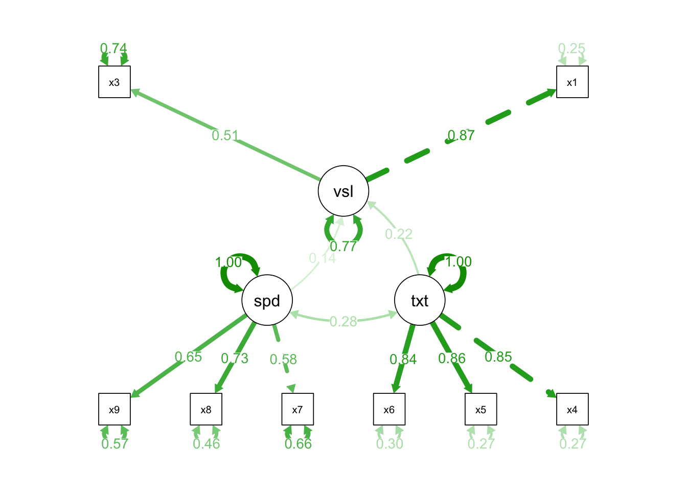
semPaths(fit, what = "path", whatLabels = "std", style = "lisrel", edge.label.cex = .9, rotation = 2, curve = 2, layoutSplit = FALSE, normalize = FALSE, height = 9, width = 6.5, residScale = 10)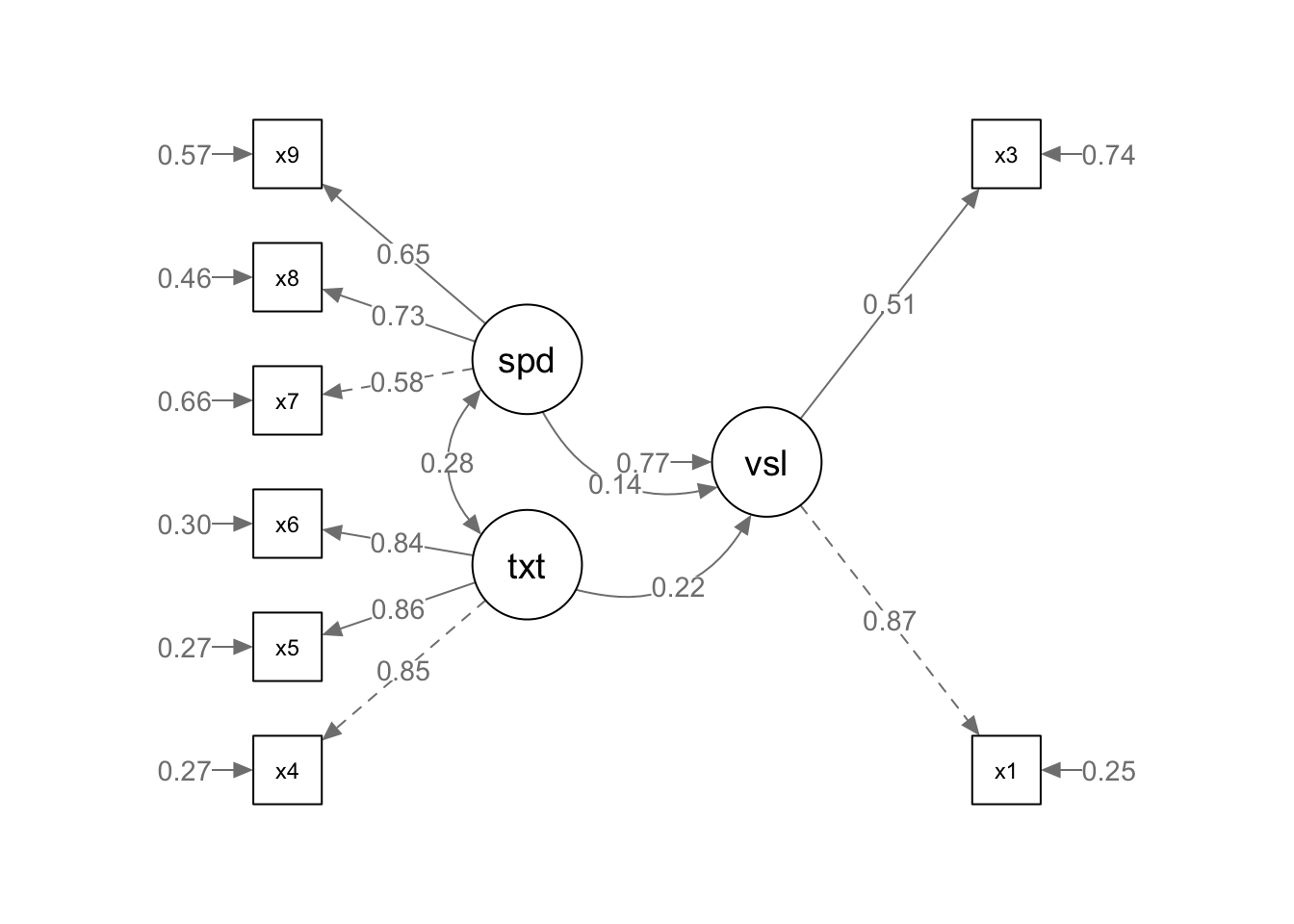
The output indicates a satisfactory fitting model despite the significant chi-square result (CFI = .93, RMSEA = .092, p = .001). Visual factors x1 and x3 loaded as expected, while x2 is approaching the lower bound for acceptable factor loading. As no items were non-significant, we might consider removing this item in a subsequent analysis to improve overall model fit. The textual and speed factor loadings were each satisfactory with the textual model holding strong consistency across each measured item (all loaded onto factor with a standardized estimate of .85 or .84). Covariances were satisfactory for this model (visual to textual is .46, visual to speed is .47, textual to speed is .28).
When we remove x2 from the model the CFI is improved at the expense of
the RMSEA value. As there are no other benefits to removing this item,
it should be retained. This model can be visualized using the
semPlot() package. The semPath() function in particular is what we
use to plot our SEM diagram. The semPaths() function takes the
following arguments. For a description of each, see
https://www.rdocumentation.org/packages/semPlot/versions/1.1.2/topics/semPaths
semPaths(object, what = "paths", whatLabels, style, layout = "tree",
  intercepts = TRUE, residuals = TRUE, thresholds = TRUE, intStyle = "multi",
  rotation = 1, curve, curvature = 1, nCharNodes = 3, nCharEdges = 3, sizeMan = 5,
   sizeLat = 8,  sizeInt = 2, sizeMan2, sizeLat2, sizeInt2, shapeMan, shapeLat,
  shapeInt = "triangle", ask, mar, title, title.color = "black", title.adj = 0.1,
  title.line = -1, title.cex = 0.8, include, combineGroups = FALSE, manifests,
  latents, groups, color, residScale, gui = FALSE, allVars = FALSE, edge.color,
  reorder = TRUE, structural = FALSE, ThreshAtSide = FALSE, thresholdColor,
  thresholdSize = 0.5, fixedStyle = 2, freeStyle = 1,
  as.expression = character(0), optimizeLatRes = FALSE, inheritColor = TRUE,
  levels, nodeLabels, edgeLabels, pastel = FALSE, rainbowStart = 0, intAtSide,
  springLevels = FALSE, nDigits = 2, exoVar, exoCov = TRUE, centerLevels = TRUE,
  panelGroups = FALSE, layoutSplit = FALSE, measurementLayout = "tree", subScale,
  subScale2, subRes = 4, subLinks, modelOpts = list(mplusStd = "std"),
  curveAdjacent = '<->', edge.label.cex = 0.6,  cardinal = "none",
  equalizeManifests = FALSE, covAtResiduals = TRUE, bifactor, optimPoints = 1:8 * (pi/4),
  ...)
## Error in eval(expr, envir, enclos): '...' used in an incorrect context6.1.1.2 Full SEM
We will be using another lavaan dataset for a Full SEM example. The
PoliticalDemocracy datasets includes 75 observations of 11 variables
that measure political democracy and industrialization in developing
countries. Variables are labeled with the following descriptions:
Political Democracy in 1960
y1: Expert ratings of the freedom of the press in 1960
y2: The freedom of political opposition in 1960
y3: The fairness of elections in 1960
y4: The effectiveness of the elected legislature in 1960
Political Democracy in 1965
y5: Expert ratings of the freedom of the press in 1965
y6: The freedom of political opposition in 1965
y7: The fairness of elections in 1965
y8: The effectiveness of the elected legislature in 1965
Level of Industrialization in 1960
x1: The gross national product (GNP) per capita in 1960
x2: The inanimate energy consumption per capita in 1960
x3: The percentage of the labor force in industry in 1960
The bold headers represent latent, unobservable variables that are quantified by the observable bullet points. Take a quick look at the dataset using any of the methods covered thus far.
str(PoliticalDemocracy)## 'data.frame': 75 obs. of 11 variables:
## $ y1: num 2.5 1.25 7.5 8.9 10 7.5 7.5 7.5 2.5 10 ...
## $ y2: num 0 0 8.8 8.8 3.33 ...
## $ y3: num 3.33 3.33 10 10 10 ...
## $ y4: num 0 0 9.2 9.2 6.67 ...
## $ y5: num 1.25 6.25 8.75 8.91 7.5 ...
## $ y6: num 0 1.1 8.09 8.13 3.33 ...
## $ y7: num 3.73 6.67 10 10 10 ...
## $ y8: num 3.333 0.737 8.212 4.615 6.667 ...
## $ x1: num 4.44 5.38 5.96 6.29 5.86 ...
## $ x2: num 3.64 5.06 6.26 7.57 6.82 ...
## $ x3: num 2.56 3.57 5.22 6.27 4.57 ...psych::describe(PoliticalDemocracy)## vars n mean sd median trimmed mad min max range skew kurtosis se
## y1 1 75 5.46 2.62 5.40 5.46 3.11 1.25 10.00 8.75 -0.09 -1.15 0.30
## y2 2 75 4.26 3.95 3.33 4.09 4.94 0.00 10.00 10.00 0.32 -1.47 0.46
## y3 3 75 6.56 3.28 6.67 6.92 4.94 0.00 10.00 10.00 -0.59 -0.72 0.38
## y4 4 75 4.45 3.35 3.33 4.33 4.94 0.00 10.00 10.00 0.12 -1.21 0.39
## y5 5 75 5.14 2.61 5.00 5.23 3.71 0.00 10.00 10.00 -0.23 -0.78 0.30
## y6 6 75 2.98 3.37 2.23 2.51 3.31 0.00 10.00 10.00 0.89 -0.47 0.39
## y7 7 75 6.20 3.29 6.67 6.47 4.94 0.00 10.00 10.00 -0.55 -0.73 0.38
## y8 8 75 4.04 3.25 3.33 3.82 4.40 0.00 10.00 10.00 0.45 -0.96 0.37
## x1 9 75 5.05 0.73 5.08 5.03 0.82 3.78 6.74 2.95 0.25 -0.75 0.08
## x2 10 75 4.79 1.51 4.96 4.85 1.53 1.39 7.87 6.49 -0.35 -0.57 0.17
## x3 11 75 3.56 1.41 3.57 3.53 1.51 1.00 6.42 5.42 0.08 -0.94 0.16A model is specified below. Run, interpret, and visualize the model.
model <- '
  # measurement model
    ind60 =~ x1 + x2 + x3
    dem60 =~ y1 + y2 + y3 + y4
    dem65 =~ y5 + y6 + y7 + y8
  # regressions
    dem60 ~ ind60
    dem65 ~ ind60 + dem60
  # residual correlations
    y1 ~~ y5
    y2 ~~ y4 + y6
    y3 ~~ y7
    y4 ~~ y8
    y6 ~~ y8
'
fit <- sem(model, data=PoliticalDemocracy)
summary(fit, fit.measures = TRUE, standardized=TRUE)
## lavaan 0.6-11 ended normally after 68 iterations
##
## Estimator ML
## Optimization method NLMINB
## Number of model parameters 31
##
## Number of observations 75
##
## Model Test User Model:
##
## Test statistic 38.125
## Degrees of freedom 35
## P-value (Chi-square) 0.329
##
## Model Test Baseline Model:
##
## Test statistic 730.654
## Degrees of freedom 55
## P-value 0.000
##
## User Model versus Baseline Model:
##
## Comparative Fit Index (CFI) 0.995
## Tucker-Lewis Index (TLI) 0.993
##
## Loglikelihood and Information Criteria:
##
## Loglikelihood user model (H0) -1547.791
## Loglikelihood unrestricted model (H1) -1528.728
##
## Akaike (AIC) 3157.582
## Bayesian (BIC) 3229.424
## Sample-size adjusted Bayesian (BIC) 3131.720
##
## Root Mean Square Error of Approximation:
##
## RMSEA 0.035
## 90 Percent confidence interval - lower 0.000
## 90 Percent confidence interval - upper 0.092
## P-value RMSEA <= 0.05 0.611
##
## Standardized Root Mean Square Residual:
##
## SRMR 0.044
##
## Parameter Estimates:
##
## Standard errors Standard
## Information Expected
## Information saturated (h1) model Structured
##
## Latent Variables:
## Estimate Std.Err z-value P(>|z|) Std.lv Std.all
## ind60 =~
## x1 1.000 0.670 0.920
## x2 2.180 0.139 15.742 0.000 1.460 0.973
## x3 1.819 0.152 11.967 0.000 1.218 0.872
## dem60 =~
## y1 1.000 2.223 0.850
## y2 1.257 0.182 6.889 0.000 2.794 0.717
## y3 1.058 0.151 6.987 0.000 2.351 0.722
## y4 1.265 0.145 8.722 0.000 2.812 0.846
## dem65 =~
## y5 1.000 2.103 0.808
## y6 1.186 0.169 7.024 0.000 2.493 0.746
## y7 1.280 0.160 8.002 0.000 2.691 0.824
## y8 1.266 0.158 8.007 0.000 2.662 0.828
##
## Regressions:
## Estimate Std.Err z-value P(>|z|) Std.lv Std.all
## dem60 ~
## ind60 1.483 0.399 3.715 0.000 0.447 0.447
## dem65 ~
## ind60 0.572 0.221 2.586 0.010 0.182 0.182
## dem60 0.837 0.098 8.514 0.000 0.885 0.885
##
## Covariances:
## Estimate Std.Err z-value P(>|z|) Std.lv Std.all
## .y1 ~~
## .y5 0.624 0.358 1.741 0.082 0.624 0.296
## .y2 ~~
## .y4 1.313 0.702 1.871 0.061 1.313 0.273
## .y6 2.153 0.734 2.934 0.003 2.153 0.356
## .y3 ~~
## .y7 0.795 0.608 1.308 0.191 0.795 0.191
## .y4 ~~
## .y8 0.348 0.442 0.787 0.431 0.348 0.109
## .y6 ~~
## .y8 1.356 0.568 2.386 0.017 1.356 0.338
##
## Variances:
## Estimate Std.Err z-value P(>|z|) Std.lv Std.all
## .x1 0.082 0.019 4.184 0.000 0.082 0.154
## .x2 0.120 0.070 1.718 0.086 0.120 0.053
## .x3 0.467 0.090 5.177 0.000 0.467 0.239
## .y1 1.891 0.444 4.256 0.000 1.891 0.277
## .y2 7.373 1.374 5.366 0.000 7.373 0.486
## .y3 5.067 0.952 5.324 0.000 5.067 0.478
## .y4 3.148 0.739 4.261 0.000 3.148 0.285
## .y5 2.351 0.480 4.895 0.000 2.351 0.347
## .y6 4.954 0.914 5.419 0.000 4.954 0.443
## .y7 3.431 0.713 4.814 0.000 3.431 0.322
## .y8 3.254 0.695 4.685 0.000 3.254 0.315
## ind60 0.448 0.087 5.173 0.000 1.000 1.000
## .dem60 3.956 0.921 4.295 0.000 0.800 0.800
## .dem65 0.172 0.215 0.803 0.422 0.039 0.039semPaths(fit, what = "path", whatLabels = "std", style = "lisrel", edge.label.cex = .9, rotation = 2, curve = 2, layoutSplit = FALSE, normalize = FALSE, height = 9, width = 6.5, residScale = 10)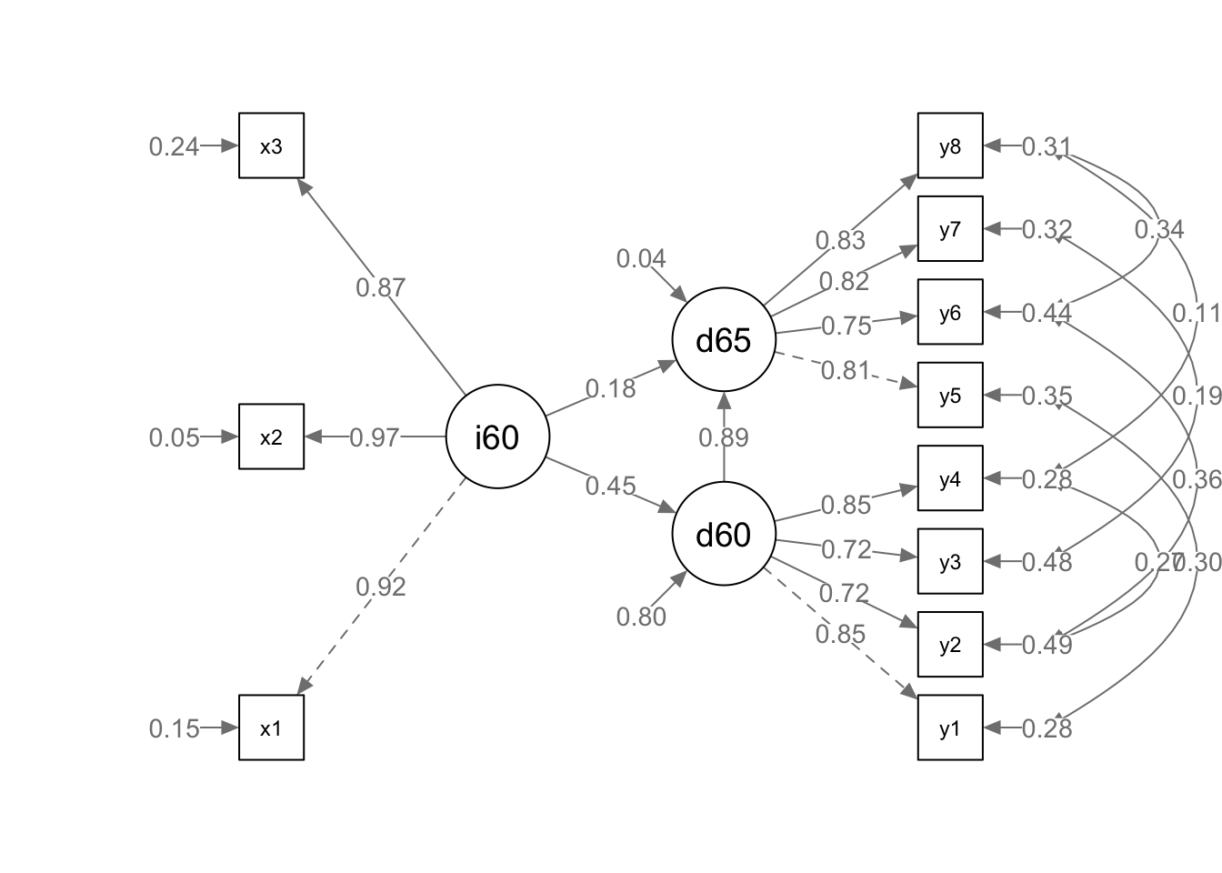
The results suggest that the model has excellent fit with a non significant chi square, a CFI of .995, and a RMSEA value .035. All factors (Ind60 x1 = .92, x2 = .97, x3 = .87; Dem60 y1 = .85, y2 = .71, y3 = .72, y4 = .85; Dem65 y5 = .81, y6 = .75, y7 = .82, y = .83) and paths (Dem60 ~ ind60 = .45; Dem65 ~ ind60(.18) + dem60(.89)) were significant and there was no evidence of colinearity in the model. Pruning would not be advisable as the model demonstrates outstanding parsimony. How do you interpret these findings on a practical level?
6.1.1.3 Mediation
We can create mediation models where intermediate variables are considered and called the mediator. We use these variables to attempt to explain the impact of an independent variable on an outcome. For instance, it is logical to deduce that past democratization of a country (d60) would predict future democratization (d65). However, it is questionable whether the industrialization of a country predicts a move toward democratization over time.
Let’s set up a mediation model to answer the research question: “To what extent does a country’s level of industrialization impact the development of political democracy over time?” Retain the same latent variables from the previous model. To create a mediation model, use the following formula:
direct effect Y ~ cX # mediator M ~ aX Y ~ bM # indirect effect (ab) ab := ab # total effect total := c + (ab)
The := operator “defines” new parameters which take on values that are
an arbitrary function of the original model parameters”
(https://lavaan.ugent.be/tutorial/mediation.html).
model <-  '
  # measurement model
    ind60 =~ x1 + x2 + x3
    dem60 =~ y1 + y2 + y3 + y4
    dem65 =~ y5 + y6 + y7 + y8

  # mediation
    dem65 ~ c*dem60
    ind60 ~ a*dem60
    dem65 ~ b*ind60

  # indirect effect (a*b)
    ab := a*b

  # total effect
    total := c + (a*b)

'
fit <- sem(model, data=PoliticalDemocracy)
summary(fit, fit.measures = TRUE, standardized=TRUE)
## lavaan 0.6-11 ended normally after 37 iterations
##
## Estimator ML
## Optimization method NLMINB
## Number of model parameters 25
##
## Number of observations 75
##
## Model Test User Model:
##
## Test statistic 72.462
## Degrees of freedom 41
## P-value (Chi-square) 0.002
##
## Model Test Baseline Model:
##
## Test statistic 730.654
## Degrees of freedom 55
## P-value 0.000
##
## User Model versus Baseline Model:
##
## Comparative Fit Index (CFI) 0.953
## Tucker-Lewis Index (TLI) 0.938
##
## Loglikelihood and Information Criteria:
##
## Loglikelihood user model (H0) -1564.959
## Loglikelihood unrestricted model (H1) -1528.728
##
## Akaike (AIC) 3179.918
## Bayesian (BIC) 3237.855
## Sample-size adjusted Bayesian (BIC) 3159.062
##
## Root Mean Square Error of Approximation:
##
## RMSEA 0.101
## 90 Percent confidence interval - lower 0.061
## 90 Percent confidence interval - upper 0.139
## P-value RMSEA <= 0.05 0.021
##
## Standardized Root Mean Square Residual:
##
## SRMR 0.055
##
## Parameter Estimates:
##
## Standard errors Standard
## Information Expected
## Information saturated (h1) model Structured
##
## Latent Variables:
## Estimate Std.Err z-value P(>|z|) Std.lv Std.all
## ind60 =~
## x1 1.000 0.669 0.920
## x2 2.182 0.139 15.714 0.000 1.461 0.973
## x3 1.819 0.152 11.956 0.000 1.218 0.872
## dem60 =~
## y1 1.000 2.201 0.845
## y2 1.354 0.175 7.755 0.000 2.980 0.760
## y3 1.044 0.150 6.961 0.000 2.298 0.705
## y4 1.300 0.138 9.412 0.000 2.860 0.860
## dem65 =~
## y5 1.000 2.084 0.803
## y6 1.258 0.164 7.651 0.000 2.623 0.783
## y7 1.282 0.158 8.137 0.000 2.673 0.819
## y8 1.310 0.154 8.529 0.000 2.730 0.847
##
## Regressions:
## Estimate Std.Err z-value P(>|z|) Std.lv Std.all
## dem65 ~
## dem60 (c) 0.864 0.113 7.671 0.000 0.913 0.913
## ind60 ~
## dem60 (a) 0.136 0.036 3.738 0.000 0.448 0.448
## dem65 ~
## ind60 (b) 0.453 0.220 2.064 0.039 0.146 0.146
##
## Variances:
## Estimate Std.Err z-value P(>|z|) Std.lv Std.all
## .x1 0.082 0.020 4.180 0.000 0.082 0.154
## .x2 0.118 0.070 1.689 0.091 0.118 0.053
## .x3 0.467 0.090 5.174 0.000 0.467 0.240
## .y1 1.942 0.395 4.910 0.000 1.942 0.286
## .y2 6.490 1.185 5.479 0.000 6.490 0.422
## .y3 5.340 0.943 5.662 0.000 5.340 0.503
## .y4 2.887 0.610 4.731 0.000 2.887 0.261
## .y5 2.390 0.447 5.351 0.000 2.390 0.355
## .y6 4.343 0.796 5.456 0.000 4.343 0.387
## .y7 3.510 0.668 5.252 0.000 3.510 0.329
## .y8 2.940 0.586 5.019 0.000 2.940 0.283
## .ind60 0.358 0.071 5.020 0.000 0.799 0.799
## dem60 4.845 1.088 4.453 0.000 1.000 1.000
## .dem65 0.115 0.200 0.575 0.565 0.026 0.026
##
## Defined Parameters:
## Estimate Std.Err z-value P(>|z|) Std.lv Std.all
## ab 0.062 0.031 2.012 0.044 0.065 0.065
## total 0.926 0.114 8.097 0.000 0.978 0.978semPaths(fit, "std", edge.label.cex = 1.0, curvePivot = TRUE)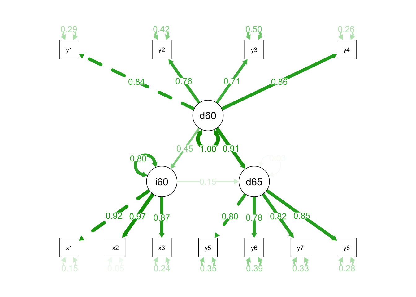
The chi-square is non significant now. The CFI is .95, and RMSEA is .101 and statistically significant. Factor structures remain intact and all paths are significant. The total effect of ind60 and dem60 explains 84% (beta weights are equivalent to r (then squared for variance explained) of the variance in dem65, however less than 1% of that variance is attributable to industrialization (p = .044). Depending on the measurement validity of this dataset, industrialization should be ruled out as a strong contributor to any change in political democracy. An additional model might be specified with other explanatory variables such as ?
6.1.1.4 Multiple Groups
If your sample size is large enough you can use lavaan to conduct
multiple group analysis. To do this add the name of the grouping
variable to group argument. The same model will be fitted to each group.
HS.model <- ' visual =~ x1 + x3
              textual =~ x4 + x5 + x6
              speed   =~ x7 + x8 + x9
              visual ~ textual'

fit <- cfa(HS.model, data = HolzingerSwineford1939, group = "school")
## Warning in lav_object_post_check(object): lavaan WARNING: some estimated ov
## variances are negativesummary(fit, fit.measures = TRUE, standardized=TRUE)## lavaan 0.6-11 ended normally after 53 iterations
##
## Estimator ML
## Optimization method NLMINB
## Number of model parameters 52
##
## Number of observations per group:
## Pasteur 156
## Grant-White 145
##
## Model Test User Model:
##
## Test statistic 107.318
## Degrees of freedom 36
## P-value (Chi-square) 0.000
## Test statistic for each group:
## Pasteur 48.124
## Grant-White 59.194
##
## Model Test Baseline Model:
##
## Test statistic 893.935
## Degrees of freedom 56
## P-value 0.000
##
## User Model versus Baseline Model:
##
## Comparative Fit Index (CFI) 0.915
## Tucker-Lewis Index (TLI) 0.868
##
## Loglikelihood and Information Criteria:
##
## Loglikelihood user model (H0) -3236.131
## Loglikelihood unrestricted model (H1) -3182.472
##
## Akaike (AIC) 6576.262
## Bayesian (BIC) 6769.032
## Sample-size adjusted Bayesian (BIC) 6604.118
##
## Root Mean Square Error of Approximation:
##
## RMSEA 0.115
## 90 Percent confidence interval - lower 0.090
## 90 Percent confidence interval - upper 0.140
## P-value RMSEA <= 0.05 0.000
##
## Standardized Root Mean Square Residual:
##
## SRMR 0.079
##
## Parameter Estimates:
##
## Standard errors Standard
## Information Expected
## Information saturated (h1) model Structured
##
##
## Group 1 [Pasteur]:
##
## Latent Variables:
## Estimate Std.Err z-value P(>|z|) Std.lv Std.all
## visual =~
## x1 1.000 1.411 1.195
## x3 0.311 0.166 1.870 0.061 0.439 0.379
## textual =~
## x4 1.000 0.949 0.826
## x5 1.177 0.101 11.668 0.000 1.117 0.855
## x6 0.870 0.076 11.455 0.000 0.825 0.836
## speed =~
## x7 1.000 0.622 0.575
## x8 1.080 0.269 4.014 0.000 0.672 0.689
## x9 0.821 0.202 4.057 0.000 0.511 0.517
##
## Regressions:
## Estimate Std.Err z-value P(>|z|) Std.lv Std.all
## visual ~
## textual 0.566 0.101 5.591 0.000 0.380 0.380
##
## Covariances:
## Estimate Std.Err z-value P(>|z|) Std.lv Std.all
## textual ~~
## speed 0.195 0.073 2.684 0.007 0.330 0.330
##
## Intercepts:
## Estimate Std.Err z-value P(>|z|) Std.lv Std.all
## .x1 4.941 0.095 52.249 0.000 4.941 4.183
## .x3 2.487 0.093 26.778 0.000 2.487 2.144
## .x4 2.823 0.092 30.689 0.000 2.823 2.457
## .x5 3.995 0.105 38.183 0.000 3.995 3.057
## .x6 1.922 0.079 24.320 0.000 1.922 1.947
## .x7 4.432 0.087 51.181 0.000 4.432 4.098
## .x8 5.563 0.078 71.214 0.000 5.563 5.702
## .x9 5.418 0.079 68.440 0.000 5.418 5.480
## .visual 0.000 0.000 0.000
## textual 0.000 0.000 0.000
## speed 0.000 0.000 0.000
##
## Variances:
## Estimate Std.Err z-value P(>|z|) Std.lv Std.all
## .x1 -0.597 0.974 -0.613 0.540 -0.597 -0.428
## .x3 1.153 0.161 7.162 0.000 1.153 0.857
## .x4 0.419 0.069 6.096 0.000 0.419 0.317
## .x5 0.460 0.086 5.367 0.000 0.460 0.269
## .x6 0.293 0.050 5.862 0.000 0.293 0.301
## .x7 0.783 0.128 6.113 0.000 0.783 0.669
## .x8 0.501 0.119 4.199 0.000 0.501 0.526
## .x9 0.716 0.103 6.922 0.000 0.716 0.733
## .visual 1.704 0.994 1.715 0.086 0.855 0.855
## textual 0.901 0.150 5.998 0.000 1.000 1.000
## speed 0.387 0.135 2.867 0.004 1.000 1.000
##
##
## Group 2 [Grant-White]:
##
## Latent Variables:
## Estimate Std.Err z-value P(>|z|) Std.lv Std.all
## visual =~
## x1 1.000 0.777 0.676
## x3 0.885 0.210 4.217 0.000 0.687 0.663
## textual =~
## x4 1.000 0.965 0.861
## x5 0.998 0.087 11.436 0.000 0.964 0.832
## x6 0.967 0.085 11.338 0.000 0.934 0.825
## speed =~
## x7 1.000 0.727 0.705
## x8 1.155 0.175 6.594 0.000 0.839 0.802
## x9 0.927 0.145 6.399 0.000 0.673 0.657
##
## Regressions:
## Estimate Std.Err z-value P(>|z|) Std.lv Std.all
## visual ~
## textual 0.471 0.101 4.677 0.000 0.585 0.585
##
## Covariances:
## Estimate Std.Err z-value P(>|z|) Std.lv Std.all
## textual ~~
## speed 0.243 0.078 3.132 0.002 0.347 0.347
##
## Intercepts:
## Estimate Std.Err z-value P(>|z|) Std.lv Std.all
## .x1 4.930 0.095 51.696 0.000 4.930 4.293
## .x3 1.996 0.086 23.195 0.000 1.996 1.926
## .x4 3.317 0.093 35.625 0.000 3.317 2.958
## .x5 4.712 0.096 48.986 0.000 4.712 4.068
## .x6 2.469 0.094 26.277 0.000 2.469 2.182
## .x7 3.921 0.086 45.819 0.000 3.921 3.805
## .x8 5.488 0.087 63.174 0.000 5.488 5.246
## .x9 5.327 0.085 62.571 0.000 5.327 5.196
## .visual 0.000 0.000 0.000
## textual 0.000 0.000 0.000
## speed 0.000 0.000 0.000
##
## Variances:
## Estimate Std.Err z-value P(>|z|) Std.lv Std.all
## .x1 0.716 0.159 4.514 0.000 0.716 0.543
## .x3 0.601 0.127 4.741 0.000 0.601 0.560
## .x4 0.325 0.065 5.036 0.000 0.325 0.259
## .x5 0.413 0.072 5.770 0.000 0.413 0.308
## .x6 0.408 0.069 5.924 0.000 0.408 0.319
## .x7 0.534 0.092 5.811 0.000 0.534 0.503
## .x8 0.390 0.099 3.932 0.000 0.390 0.357
## .x9 0.598 0.091 6.537 0.000 0.598 0.569
## .visual 0.396 0.140 2.839 0.005 0.657 0.657
## textual 0.932 0.152 6.138 0.000 1.000 1.000
## speed 0.528 0.127 4.156 0.000 1.000 1.000semPaths(fit, "std", edge.label.cex = 1.0, rotation = 2, curvePivot = TRUE)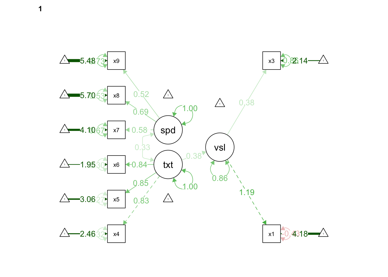
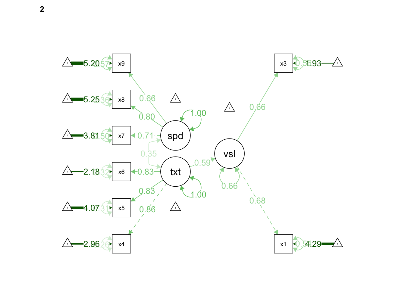
The x2 variable at the Pasteur school did not load onto the visual achievement factor. We can retool our questionnaire or consider the study validity to fix this, but for now let’s just remove it from the model again. Once we do that we can see that the x1 and x3 items are loading very differently onto the visual factor, though both items meet the threshold of .40. What would you do if this was your study?
6.1.1.5 Measurement Invariance
You can also test for measurement invariance across the grouping
variable using the measurmentInvariance() function which “performs a
number of multiple group analyses in a particular sequence, with
increasingly more restrictions on the
parameters”(https://lavaan.ugent.be/tutorial/groups.html). Load the
semTools library to use this function.
There are four types of measurment invariance.
The first is equal form configural invariance, which assumes the factor structures (number of items) and patterns (relationships between factors) are identical across groups. The second is equal loadings (metric invariance), which assumes that factor loadings (extent which each item loads onto factors) are equal across groups. The third is equal intercepts (scalar invariance), which assumes that the intercepts of observed scores are equal across groups. Finally, equal residual variances (strict invariance) assumes that the residual variances of observed paths are equal across groups.
#install.packages('semTools')
library(semTools)
measurementInvariance(model = HS.model,
                      data = HolzingerSwineford1939,
                      group = "school")
##
## Measurement invariance models:
##
## Model 1 : fit.configural
## Model 2 : fit.loadings
## Model 3 : fit.intercepts
## Model 4 : fit.means
##
## Chi-Squared Difference Test
##
## Df AIC BIC Chisq Chisq diff Df diff Pr(>Chisq)
## fit.configural 36 6576.3 6769.0 107.32
## fit.loadings 41 6576.3 6750.5 117.35 10.030 5 0.07439 .
## fit.intercepts 46 6600.7 6756.4 151.78 34.431 5 1.954e-06 ***
## fit.means 49 6638.2 6782.7 195.21 43.431 3 1.993e-09 ***
## ---
## Signif. codes: 0 '***' 0.001 '**' 0.01 '*' 0.05 '.' 0.1 ' ' 1
##
##
## Fit measures:
##
## cfi rmsea cfi.delta rmsea.delta
## fit.configural 0.915 0.115 NA NA
## fit.loadings 0.909 0.111 0.006 0.003
## fit.intercepts 0.874 0.124 0.035 0.012
## fit.means 0.826 0.141 0.048 0.017This model assesses the four measurement invariance types across the grouping variable ‘school’ in the HS dataset. No model met the acceptable threshold for RMSEA. Judging by CFI alone, which is not always advisable, form, loadings, and intercept models demonstrate good fit. Thus, each school represented in the HS dataset can be assumed to be equal in these respects, but fail to demonstrate strict invariance. These statistics might be used to validate this particular measure as congruent across different groups of students.
6.2 Case Study
In our case study we will be modeling data from Holzer et al.’s (2021) published data on self regulated learning and well being. The abstract and source are pasted below.
“In the wake of COVID-19, university students have experienced fundamental changes of their learning and their lives as a whole. The present research identifies psychological characteristics associated with students’ well-being in this situation. We investigated relations of basic psychological need satisfaction (experienced competence, autonomy, and relatedness) with positive emotion and intrinsic learning motivation, considering self-regulated learning as a moderator. Self-reports were collected from 6,071 students in Austria (Study 1) and 1,653 students in Finland (Study 2). Structural equation modeling revealed competence as the strongest predictor for positive emotion. Intrinsic learning motivation was predicted by competence and autonomy in both countries and by relatedness in Finland. Moderation effects of self-regulated learning were inconsistent, but main effects on intrinsic learning motivation were identified. Surprisingly, relatedness only exerted a minor effect on positive emotion. The results inform strategies to promote students’ well-being through distance-learning, mitigating negative effects of the situation.”
The authors saved the data in an SPSS file (.sav). Let’s use the haven library to read and convert the data file into a dataset.
#install.packages('haven')
library(haven)

path = file.path("semcasestudy.sav")
dataset = read_sav(path)
Examine the dataset using str(), summary() or DataExplorer::create_report()
dataset## # A tibble: 7,724 × 39
## country gender age sr1 sr2 sr3 comp1 comp2 comp3 auto1
## <dbl+l> <dbl+l> <dbl> <dbl+l> <dbl+l> <dbl+l> <dbl+l> <dbl+l> <dbl+l> <dbl+l>
## 1 0 [Aus… 1 [fem… 36 5 [str… 4 [dis… 2 [agr… 2 [agr… 3 [som… 3 [som… 3 [som…
## 2 0 [Aus… 2 [mal… 36 4 [dis… 4 [dis… 1 [str… 4 [dis… 4 [dis… 3 [som… 4 [dis…
## 3 0 [Aus… 2 [mal… 36 1 [str… 1 [str… 1 [str… 3 [som… 4 [dis… 2 [agr… 5 [str…
## 4 0 [Aus… 2 [mal… 36 1 [str… 2 [agr… 1 [str… 2 [agr… 2 [agr… 2 [agr… 4 [dis…
## 5 0 [Aus… 1 [fem… 36 1 [str… 1 [str… 3 [som… 3 [som… 2 [agr… 3 [som… 4 [dis…
## 6 0 [Aus… 1 [fem… 36 1 [str… 1 [str… 1 [str… 2 [agr… 2 [agr… 2 [agr… 3 [som…
## 7 0 [Aus… 1 [fem… 36 2 [agr… 2 [agr… 2 [agr… 4 [dis… 3 [som… 3 [som… 4 [dis…
## 8 0 [Aus… 1 [fem… 36 2 [agr… 1 [str… 1 [str… 2 [agr… 1 [str… 2 [agr… 3 [som…
## 9 0 [Aus… 3 [oth… 36 5 [str… 4 [dis… 2 [agr… 3 [som… 1 [str… 3 [som… 4 [dis…
## 10 0 [Aus… 1 [fem… 36 4 [dis… 3 [som… 2 [agr… 3 [som… 2 [agr… 3 [som… 3 [som…
## # … with 7,714 more rows, and 29 more variables: auto2 <dbl+lbl>,
## # auto3 <dbl+lbl>, pa1 <dbl+lbl>, pa2 <dbl+lbl>, pa3 <dbl+lbl>,
## # lm1 <dbl+lbl>, lm2 <dbl+lbl>, lm3 <dbl+lbl>, gp1 <dbl+lbl>, gp2 <dbl+lbl>,
## # gp3 <dbl+lbl>, sr1.rec <dbl+lbl>, sr2.rec <dbl+lbl>, sr3.rec <dbl+lbl>,
## # comp1.rec <dbl+lbl>, comp2.rec <dbl+lbl>, comp3.rec <dbl+lbl>,
## # auto1.rec <dbl+lbl>, auto2.rec <dbl+lbl>, auto3.rec <dbl+lbl>,
## # pa1.rec <dbl+lbl>, pa2.rec <dbl+lbl>, pa3.rec <dbl+lbl>, …Subjective Well-Being (SWB) describes “how people experience the quality of their lives, which includes both emotional reactions and cognitive judgements”, encompassing moods, emotions, and satisfaction in general and specific areas of life (Martela & Ryan, 2015). Situations outside of our control, such as natural disasters or pandemics, have a significant impact on SWB. For instance, the COVID-19 outbreak has been associated with a 74% dip in SWB in China, a phenomenon also felt across Europe and the United States.
Self regulation style is represented by a motivational spectrum, developed by Deci & Ryan (2000) where students exhibit behavior regulation styles as they perceive motivational influences from either external or internal sources. This spectrum ranges from extrinsic to intrinsic. For instance, financial gain may serve as an extrinsic regulator, as in the salary a person earns motivates them to come to work every day, while the pressure of a duty or a job is an example of introjected regulation, where a person feels they must complete an action due to external pressure, often from other people or the environment. Identified regulation occurs when a person’s identity intersects with an expected set of tasks for success, for instance, I am a musician, so I have to practice. On the far end of the spectrum, intrinsic regulation is self-sustaining, and catalyzed by an identified interest and curiosity for a task. Hundreds of studies across multiple continents suggest that the satisfaction of basic psychological needs can encourage students to move along the spectrum towards intrinsic regulation, where growth, learning, and skill acquisition become self-regulated processes. To practice these skills, follow the directions below.
Considering the theory behind these data, start drafting some research questions. I tend to find that when constructing initial models, it is imperative to draw my thinking on paper and construct model syntax.
Use the code box below to specify your own model based on Holzer et al.’s (2021) dataset. You may need to create composite indexes using multiple subscales of observed variables before specifying your model. If you aren’t sure where to start, go back to the abstract at the start of the case study for evidence of Holzer et al.’s model specifications. Also see the codebook titled ‘HolzerReadme’ at https://osf.io/6jb9t/ within this short course’s folder. Hint: Most items were collected with strongly agree coded as 1, with strongly disagree coded as 5. All items have been recoded to match magnitude with numerical order. These items are labeled as item.rec.
Run the model and interpret the results.
Visualize the model.
Do you need to specify a new model? Do any paths need to be pruned? Write new formulas below. Then run, visualize and interpret the model.
Does your model hold across Austrian and Finnish populations? Group your model by country to see the output of each model, then run a test of measurement invariance on your model.
Make a few notes here regarding potential next steps for research. Consider how the COVID-19 pandemic might impact the measured relationships.
Specify and run a mediation model including variables in the Holzer et al. (2021) dataset.
6.3 Review
In this chapter we introduced SEM concepts and methods. To make sure you understand this material, there is a practice assessment to go along with this chapter at https://jayholster.shinyapps.io/SEMinRAssessment/
6.4 References
Deci, E. L., & Ryan, R. M. (2000) The “What and”Why” of goal pursits: Human needs and the self-determination of behavior. Psychological Inquiry, 11(4), 227–268.
Epskamp, S. (2015). semPlot: Unified visualizations of structural equation models. Structural Equation Modeling, 22(3), 474–483. <https://doi.org/10.1080/10705511.2014.937847>
Holzer, J., Lüftenegger, M., Korlat, S., Pelikan, E., Salmela-Aro, K., Spiel, C., & Schober, B. (2021). Higher dducation in times of COVID-19: University students’ basic need satisfaction, self-regulated learning and well-being. Ann Arbor, MI: Inter-university Consortium for Political and Social Research [distributor]. https://doi.org/10.3886/E133601V1
Martela, F, & Ryan, R. (2015). The benefits of benevolence: Basic psychological needs, beneficence, and the enhancement of well-being. Journal of Personality, 84(6), 750–764. https://doi.org/10.1111/jopy.12215
Rosseel, Y. (2012). lavaan: An R Package for Structural Equation Modeling. Journal of Statistical Software, 48(2), 1–36. [https://doi.org/[10.18637/jss.v048.i02](https://doi.org/[10.18637/jss.v048.i02)](https://doi.org/%5B10.18637/jss.v048.i02){.uri}.
6.4.1 R Short Course Series
Video lectures of each guidebook chapter can be found at https://osf.io/6jb9t/. For this chapter, find the follow the folder path Structural Equation Modeling in R -> AY 2021-2022 Spring and access the video files, r markdown documents, and other materials for each short course.
6.4.2 Acknowledgements
This guidebook was created with support from the Center for Research Data and Digital Scholarship and the Laboratory for Interdisciplinary Statistical Analaysis at the University of Colorado Boulder, as well as the U.S. Agency for International Development under cooperative agreement #7200AA18CA00022. Individuals who contributed to materials related to this project include Jacob Holster, Eric Vance, Michael Ramsey, Nicholas Varberg, and Nickoal Eichmann-Kalwara.