Chapter 4 Foundations of Statistical Analysis
Quantitative methods suggest that rules of probability can determine whether observed differences within or between groups in a sample represents a real difference in a population. These differences are communicated in terms of statistics, which are essentially numbers that describe characteristics of data. These characteristics are measured, described, compared, and modeled in varied ways. However, all statistical analysis share a similar aim—to make meaning from quantitative data or to explain some observed phenomena (e.g, current status of a variable, relationships between variables, effects between variables).
As statistical analysis is embedded in the scientific method, the R user might consider the research process at large before interacting with R. When analyzing data it is helpful to hold a genuine desire to understand a topic, be aware of and control your biases, resist simplistic or convenient explanations for relationships, and employ systematic peer-reviewed methods. When asking and investigating research questions, it is suggested to set aside your personal beliefs and experiences regarding the data. Additionally, be willing to adopt rational perspectives on your data while suspending disbelief about findings that are contrary to your expectations or beliefs.
In this and the following chapter, you will be guided through methods that will support many types of statistical analyses. For instance, you will learn how to determine the prevalence of a phenomenon, explore underlying factors, test interventions, test group differences, and explore multivariate approaches to statistical analysis.
4.1 Descriptive Statistics
Descriptive statistics provide a (for lack of a better term) description of what is observed in collected data—whereby measures of centrality and variability are our main tools for understanding. These are oftentimes referred to as summary statistics. We use descriptive statistics to assess the characteristics of participants, which supports the ability to make statements regarding make the generalizability of the sample to the overall population or other context.
Measures of central tendency are used to describe data with a single number. For instance, the mean represents the average of all of each of the individual data within a set.
mean(mtcars$mpg)## [1] 20.09062The median describes the point at which 50% of cases in a distribution fall below and 50% fall above.
median(mtcars$mpg)## [1] 19.2Variability is the amount of spread or dispersion in a set of scores. Knowing the extent to which data varies allows researchers to compare groups within data effectively and accurately.
Assessments of variability provide a representation of the amount of dispersion within a distribution from a measure of central tendency. For instance, range displays the lowest and highest score in a vector.
range(mtcars$mpg)## [1] 10.4 33.9Standard deviation represents the average score deviation from the mean.
sd(mtcars$mpg)## [1] 6.026948Variance is the square of the standard deviation.
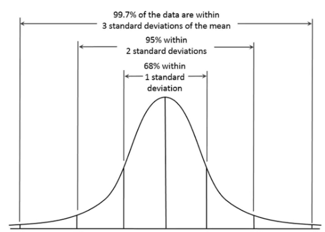
var(mtcars$mpg)## [1] 36.3241In reference to the distribution of the data, standard deviations tell us where scores generally fall. SD is often reported alongside the mean (e.g., M = 7, SD = 1.5). With these numbers, we can ascertain that 68% of scores will fall between 5.5 and 8.5, and 95% of scores fall between 4 and 10. Furthermore, we can ascertain with a normal distribution that about 99% of scores might fall between 2.5 and 12.5.
These association between means, standard deviations, and normal distributions parameterize the probability of future observations on a similar measure. Many of the most common statistical tests we use are conceived of assuming this parametric concept—rationalizing the assumption that observations will be normally distributed.
As exemplified above, data that meet this assumption tend to have around 68% of data points falling between +-1 standard deviation of the mean, and 95% of data falling between +-2 standard deviations of the mean. Furthermore, normality tends to be met when the distribution curve is peaked at the mean and has only one mode. Additionally, the curve in a normal distribution should be symmetrical on both sides of the mean, median, and mode while having asymptotic tails (tails curve but do not approach the axis; no 100s or zeros).
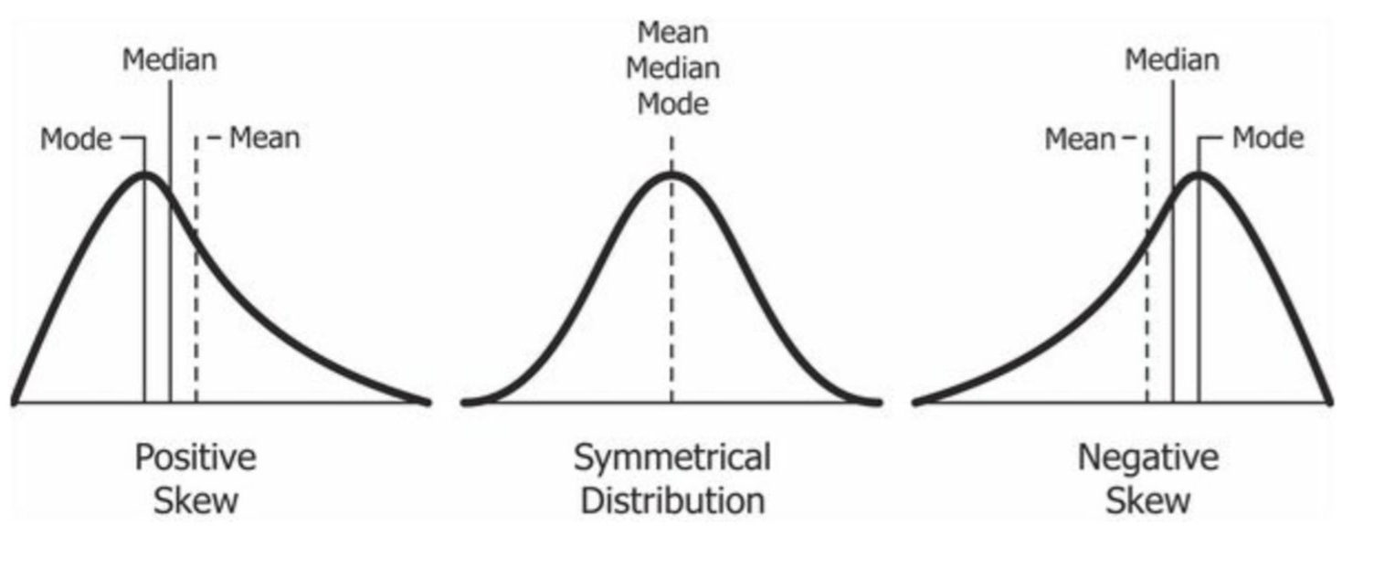
A distribution is skewed, or has skewness, positively or negatively when there is longer tail on one of the distribution. A longer tail on the right tends to indicate a smaller number of data points at the higher end of the distribution—a positive skew. A shorter tail on the right indicates a larger number of data points on the high end of the distribution—a negative skew.
One helpful rule of thumb is that if the mean is greater than the median the distribution likely has a positive skew. Conversely, if the mean is less than the median, the distribution likely has a negative skew. See the figure below for an illustration of each distribution.
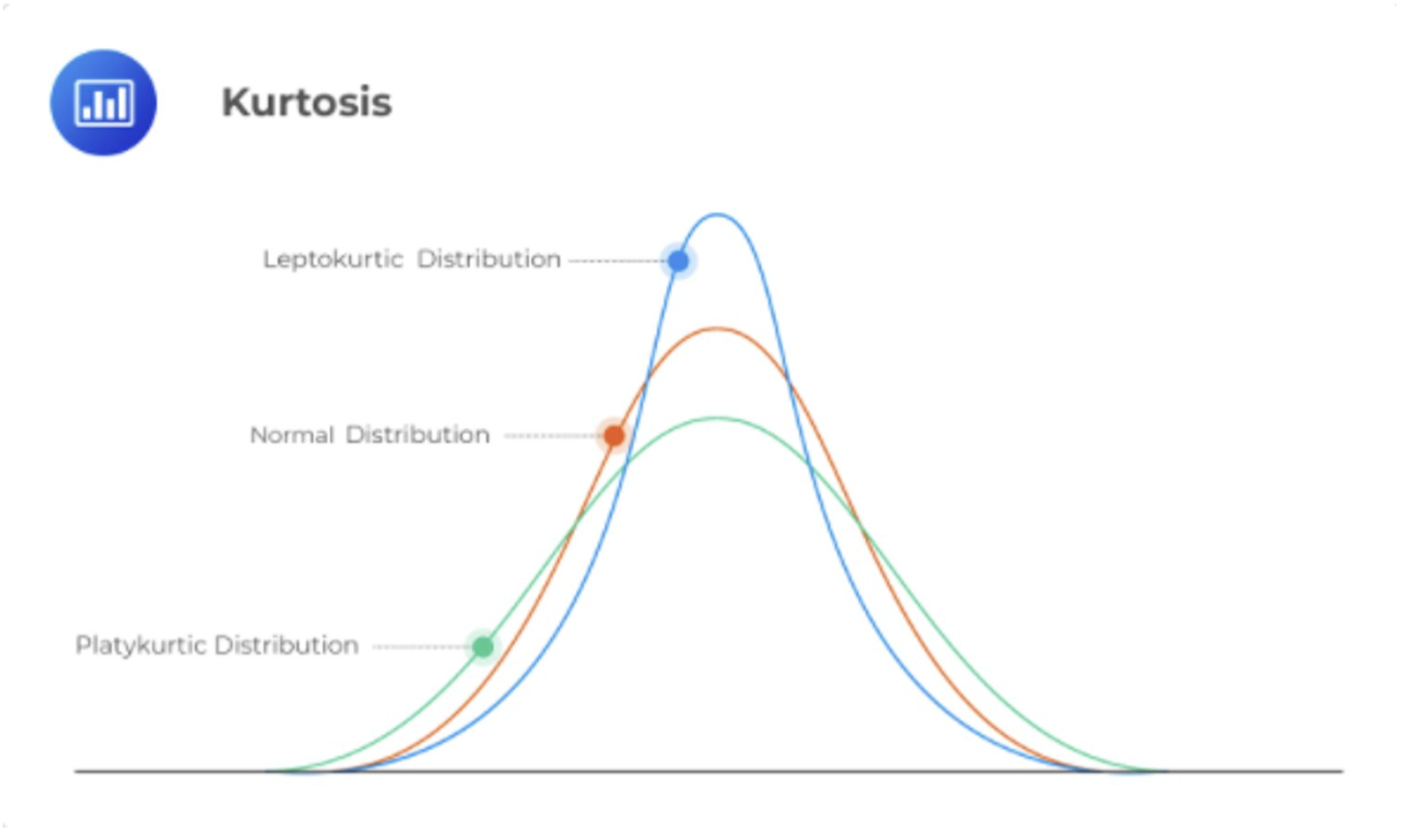
The smaller the standard deviation and variance, the higher the level of agreement, or similarity, in response or scores. When agreement or similarity in scores is very high a distribution may be leptokurtic—having low variance (i.e., small standard deviations). When scores are very broad high variance may create a platykurtic distribution. These are represented within the concept of kurtosis. Kurtosis will be assessed alongside skewness in a few paragraphs.
There are several ways to assess for the assumption of normality. Some
researchers prefer to visually assess histograms. Some like to compare
means and medians within the context of standard deviations. The most
reliable, and mathematically-based, may be a Shapiro-Wilk test. A
non-significant Shapiro-Wilk outcome will provide support of a normal
distribution as test significance can be practically interpreted to
suggest that the distribution is significantly different than a vector
that is normally distributed. For instance, as the p value exceeds .05
when applied to the mtcars mpg column the miles per gallon variable can
be interpreted as normally distributed across the vector. Use the
function shapiro.test()
shapiro.test(mtcars$mpg)##
## Shapiro-Wilk normality test
##
## data: mtcars$mpg
## W = 0.94756, p-value = 0.1229You can also examine the influence of kurtosis and skewness values using
the psych::describe() function. Interpretations of skewness and
kurtosis values differ from field to field, but generally you can assume
a normal distribution if these values fall within -3 and +3.
psych::describe(mtcars$mpg)## vars n mean sd median trimmed mad min max range skew kurtosis se
## X1 1 32 20.09 6.03 19.2 19.7 5.41 10.4 33.9 23.5 0.61 -0.37 1.074.1.1 Case Study Part One
We are going to utilize the mtcars dataset to apply descriptive statistical concepts using R. The dataset includes information regarding fuel consumption and 10 other aspects of automobile design and performance across 32 automobiles.
Put otherwise, mtcars is a data frame with 32 observations of 11
(numeric) variables. These include:
- Miles/(US) gallon (mpg)
- Number of cylinders (cyl)
- Displacement (disp)
- Gross horsepower (hp)
- Rear axle ratio (drat)
- Weight in 1000 lbs (wt)
- 1/4 mile time (qsec)
- Engine (0 = V-shaped, 1 = straight) (vs)
- Transmission (0 = automatic, 1 = manual) (am)
- Number of forward gears (gear)
- Number of carburetors (carb)
First, load the tidyverse library and examine the dataset.
library(tidyverse, quiet = T)
data(mtcars) # bring mtcars dataset into environment
str(mtcars) #use the str() function to examine the structure of the data frame.
## 'data.frame': 32 obs. of 11 variables:
## $ mpg : num 21 21 22.8 21.4 18.7 18.1 14.3 24.4 22.8 19.2 ...
## $ cyl : num 6 6 4 6 8 6 8 4 4 6 ...
## $ disp: num 160 160 108 258 360 ...
## $ hp : num 110 110 93 110 175 105 245 62 95 123 ...
## $ drat: num 3.9 3.9 3.85 3.08 3.15 2.76 3.21 3.69 3.92 3.92 ...
## $ wt : num 2.62 2.88 2.32 3.21 3.44 ...
## $ qsec: num 16.5 17 18.6 19.4 17 ...
## $ vs : num 0 0 1 1 0 1 0 1 1 1 ...
## $ am : num 1 1 1 0 0 0 0 0 0 0 ...
## $ gear: num 4 4 4 3 3 3 3 4 4 4 ...
## $ carb: num 4 4 1 1 2 1 4 2 2 4 ...Let’s do some dataset manipulation before diving into analysis. Remember
our pipe operator %>%? It’s going to help us get rid of a column using
the select() function, and create a new column using the mutate()
function. You can read the following code as: “Assign new object mtcars
as old dataset mtcars where everything but drat is selected. Then wt is
divided by qsec using the mutate function to create a new column called
wtqsec_ratio.”
mtcars <- mtcars %>% select(-drat) %>% mutate(wtqsec_ratio = wt/qsec)When examining the structure of the data frame, note that the columns
vs, am, cyl, gear, and carb are listed as numeric when in actuality they
are factor/categorical variables. Use mutate() and as.ordered() to
set numerical vectors as ordered factors. Then, use the recode()
function to label each factor level with the appropriate string for
engine type. Finally, reexamine the structure to see evidence of the
updates.
mtcars <- mtcars %>%
  mutate(cyl = as.ordered(cyl), gear = as.ordered(gear), carb = as.ordered(carb))

mtcars <- mtcars %>%
  mutate(vs = recode_factor(vs, `0` = "v-shaped", `0.5` = 'v-shaped', `1` = "straight"),
        am = recode_factor(am, `0` = "automatic", `1` = "manual"))

str(mtcars)
## 'data.frame': 32 obs. of 11 variables:
## $ mpg : num 21 21 22.8 21.4 18.7 18.1 14.3 24.4 22.8 19.2 ...
## $ cyl : Ord.factor w/ 3 levels "4"<"6"<"8": 2 2 1 2 3 2 3 1 1 2 ...
## $ disp : num 160 160 108 258 360 ...
## $ hp : num 110 110 93 110 175 105 245 62 95 123 ...
## $ wt : num 2.62 2.88 2.32 3.21 3.44 ...
## $ qsec : num 16.5 17 18.6 19.4 17 ...
## $ vs : Factor w/ 2 levels "v-shaped","straight": 1 1 2 2 1 2 1 2 2 2 ...
## $ am : Factor w/ 2 levels "automatic","manual": 2 2 2 1 1 1 1 1 1 1 ...
## $ gear : Ord.factor w/ 3 levels "3"<"4"<"5": 2 2 2 1 1 1 1 2 2 2 ...
## $ carb : Ord.factor w/ 6 levels "1"<"2"<"3"<"4"<..: 4 4 1 1 2 1 4 2 2 4 ...
## $ wtqsec_ratio: num 0.159 0.169 0.125 0.165 0.202 ...Base R comes with a variety of functions for descriptive statistics,
including mean, sd, var, min, max, median, range, and
quantile. These can be used on specific variables in a data frame, or
to all columns or rows in the data frame using the apply function. The
X argument below represents the dataset or array to which functions will
be applied. The 2 tells R to look at the columns, whereas 1 would
indicate that a function would be applied to rows. The FUN argument
calls the specific function to apply, and na.rm denotes whether
missing data should be removed or not.
apply(X = mtcars, MARGIN = 2, FUN = min, na.rm = TRUE) ## mpg cyl disp hp wt qsec
## "10.4" "4" " 71.1" " 52" "1.513" "14.50"
## vs am gear carb wtqsec_ratio
## "straight" "automatic" "3" "1" "0.08720302"The psych library includes helpful descriptive statistics functions.
Use psych’s describe() function to see the descriptive statistics we
previously examined in one table.
#install.packages('psych')
library(psych)
psych::describe(mtcars)
## vars n mean sd median trimmed mad min max range
## mpg 1 32 20.09 6.03 19.20 19.70 5.41 10.40 33.90 23.50
## cyl* 2 32 2.09 0.89 2.00 2.12 1.48 1.00 3.00 2.00
## disp 3 32 230.72 123.94 196.30 222.52 140.48 71.10 472.00 400.90
## hp 4 32 146.69 68.56 123.00 141.19 77.10 52.00 335.00 283.00
## wt 5 32 3.22 0.98 3.33 3.15 0.77 1.51 5.42 3.91
## qsec 6 32 17.85 1.79 17.71 17.83 1.42 14.50 22.90 8.40
## vs* 7 32 1.44 0.50 1.00 1.42 0.00 1.00 2.00 1.00
## am* 8 32 1.41 0.50 1.00 1.38 0.00 1.00 2.00 1.00
## gear* 9 32 1.69 0.74 2.00 1.62 1.48 1.00 3.00 2.00
## carb* 10 32 2.72 1.37 2.00 2.65 1.48 1.00 6.00 5.00
## wtqsec_ratio 11 32 0.18 0.06 0.18 0.18 0.07 0.09 0.31 0.22
## skew kurtosis se
## mpg 0.61 -0.37 1.07
## cyl* -0.17 -1.76 0.16
## disp 0.38 -1.21 21.91
## hp 0.73 -0.14 12.12
## wt 0.42 -0.02 0.17
## qsec 0.37 0.34 0.32
## vs* 0.24 -2.00 0.09
## am* 0.36 -1.92 0.09
## gear* 0.53 -1.07 0.13
## carb* 0.35 -0.95 0.24
## wtqsec_ratio 0.27 -0.70 0.01Use the psych function describeBy() and the argument group to see
summary statistics grouped by any variable. The code below groups by
transmission, where automatic = 0 and manual = 1). The use of double
colons :: tells R to use the function from this specific package and
not any other describeBy() function from packages other than psych.
psych::describeBy(mtcars, group='am') # summary statistics by grouping variable##
## Descriptive statistics by group
## am: automatic
## vars n mean sd median trimmed mad min max range
## mpg 1 19 17.15 3.83 17.30 17.12 3.11 10.40 24.40 14.00
## cyl* 2 19 2.47 0.77 3.00 2.53 0.00 1.00 3.00 2.00
## disp 3 19 290.38 110.17 275.80 289.71 124.83 120.10 472.00 351.90
## hp 4 19 160.26 53.91 175.00 161.06 77.10 62.00 245.00 183.00
## wt 5 19 3.77 0.78 3.52 3.75 0.45 2.46 5.42 2.96
## qsec 6 19 18.18 1.75 17.82 18.07 1.19 15.41 22.90 7.49
## vs* 7 19 1.37 0.50 1.00 1.35 0.00 1.00 2.00 1.00
## am* 8 19 1.00 0.00 1.00 1.00 0.00 1.00 1.00 0.00
## gear* 9 19 1.21 0.42 1.00 1.18 0.00 1.00 2.00 1.00
## carb* 10 19 2.74 1.15 3.00 2.76 1.48 1.00 4.00 3.00
## wtqsec_ratio 11 19 0.21 0.05 0.21 0.21 0.04 0.12 0.31 0.18
## skew kurtosis se
## mpg 0.01 -0.80 0.88
## cyl* -0.95 -0.74 0.18
## disp 0.05 -1.26 25.28
## hp -0.01 -1.21 12.37
## wt 0.98 0.14 0.18
## qsec 0.85 0.55 0.40
## vs* 0.50 -1.84 0.11
## am* NaN NaN 0.00
## gear* 1.31 -0.29 0.10
## carb* -0.14 -1.57 0.26
## wtqsec_ratio 0.38 -0.68 0.01
## ------------------------------------------------------------
## am: manual
## vars n mean sd median trimmed mad min max range
## mpg 1 13 24.39 6.17 22.80 24.38 6.67 15.00 33.90 18.90
## cyl* 2 13 1.54 0.78 1.00 1.45 0.00 1.00 3.00 2.00
## disp 3 13 143.53 87.20 120.30 131.25 58.86 71.10 351.00 279.90
## hp 4 13 126.85 84.06 109.00 114.73 63.75 52.00 335.00 283.00
## wt 5 13 2.41 0.62 2.32 2.39 0.68 1.51 3.57 2.06
## qsec 6 13 17.36 1.79 17.02 17.39 2.34 14.50 19.90 5.40
## vs* 7 13 1.54 0.52 2.00 1.55 0.00 1.00 2.00 1.00
## am* 8 13 2.00 0.00 2.00 2.00 0.00 2.00 2.00 0.00
## gear* 9 13 2.38 0.51 2.00 2.36 0.00 2.00 3.00 1.00
## carb* 10 13 2.69 1.70 2.00 2.55 1.48 1.00 6.00 5.00
## wtqsec_ratio 11 13 0.14 0.05 0.13 0.14 0.05 0.09 0.24 0.16
## skew kurtosis se
## mpg 0.05 -1.46 1.71
## cyl* 0.87 -0.90 0.22
## disp 1.33 0.40 24.19
## hp 1.36 0.56 23.31
## wt 0.21 -1.17 0.17
## qsec -0.23 -1.42 0.50
## vs* -0.14 -2.13 0.14
## am* NaN NaN 0.00
## gear* 0.42 -1.96 0.14
## carb* 0.54 -1.25 0.47
## wtqsec_ratio 0.62 -0.90 0.01Analyze frequency or count data for various groups using the table()
function. The first line of code will create a table of counts
disaggregated by transmission type and number of gears. The second line
of code modifies the mtcars object to be grouped by transmission and
gear, then summarizes each into a proportion of the entire population of
cars as column ‘prop’ The spread() function is used to display the
data of interest based on established groups.
table(mtcars$am, mtcars$gear)##
## 3 4 5
## automatic 15 4 0
## manual 0 8 5mtcars %>% group_by(am, gear) %>% summarise(prop = n()/nrow(mtcars)) %>% spread(gear, prop)## `summarise()` has grouped output by 'am'. You can override using the `.groups`
## argument.## # A tibble: 2 × 4
## # Groups: am [2]
## am `3` `4` `5`
## <fct> <dbl> <dbl> <dbl>
## 1 automatic 0.469 0.125 NA
## 2 manual NA 0.25 0.1564.2 Correlational Statistics
Using contingency tables such as the first in the previous code chunk, we can run a Chi Square or Fisher’s exact test to see whether these categorical variables are independent. The null hypothesis for each of these tests is that there is no relationship between transmission type and the number of gears in a car. What do our results suggest?
tb2 <- table(mtcars$am, mtcars$gear)
chisq.test(tb2)
##
## Pearson's Chi-squared test
##
## data: tb2
## X-squared = 20.945, df = 2, p-value = 2.831e-05fisher.test(tb2)##
## Fisher's Exact Test for Count Data
##
## data: tb2
## p-value = 2.13e-06
## alternative hypothesis: two.sidedBoth tests indicate that the null hypothesis should be rejected, thus suggesting that there is a relationship between transmission type and the number of gears in a car. These tests are examples of correlational statistics, as they are measuring the association between two variables, or the extent to which they co-relate.
4.2.1 How Correlation Works
Correlation implies the desire to find a pattern or relationship between variables (e.g., What is the relationship between X and Y?). Correlation coefficients are returned as number between -1 and 1. This number tells us about the strength of the relationship between the two variables. Correlational analysis is commonly employed in survey studies as an additional analysis step beyond basic descriptive statistics.
Correlational design refers to a type of study that has the appearance of an experiment (e.g., dependent and independent variables, interventions, and even random sampling), but lacks true causality. These designs are used when the manipulation of variables may not be possible or ethical (e.g., the effects of texting while driving; effect of homelessness on student achievement). Additionally, correlational research designs can be used as a precursor to an experiment (e.g., determining what variables are correlated with student effort before trying to conduct an experiment designed to improve student effort among adolescents).
4.2.2 Correlation, not Causation?
The maxim, “correlation does not imply causation” is frequently stated, but what does it mean? In essence, finding a correlation between two variables does not establish a causal relationship. To do this, we need to know the underlying directionality/ordering of the relationship and rule out confounding variables that might explain the relationship. For example, a strong positive correlation exists between total revenue generated by arcades and computer science doctorates awarded. However, one of these events did not not cause the other.
4.2.3 Statistical Significance
The concept of statistical significance reflects that our findings are likely not due to chance, and that if we reject a null hypothesis (I.e., find a significant difference), it is likely that the same difference will hold true for the entire population. Findings are either statistical or not, (at the alpha level you set .01, .05, .10). Nonsignificant results are just as informative as significant results.
For instance, if you set your apriori alpha level to .05 for a correlation test that measures alignment of math and music performance scores and find a strong positive and significant correlation (r = .71, p = .03) there is only a 3% probability that the evidenced correlation is due to chance or some extreme, uncontrollable event. Put otherwise, the evidence for the correlation is larger than can reasonably be explained as a chance occurrence.
4.2.4 Choosing the Right Test
There are several different correlational approaches to use. See the table below for a breakdown of each correlational test and when to use it.
| Test | R Function | When to use it |
|---|---|---|
| Chi-S quare | chisq.test() |
|
| Spear man’s Rho | co r.test (method = "spearman") |
|
| Pear son’s R | c or.test (method = "pearson") |
|
4.2.5 Case Study Part Two
To continue the original case study, create a plot of displacement and
miles per gallon. There appears to be a moderate to strong negative
correlation. Use the cor.test() base R function to see correlation
coefficients and related statistical output. If your data require
nonparametric analysis, use method = spearman to call Spearman’s Rho.
ggplot(mtcars, aes(x = disp, y = mpg)) +
  geom_point()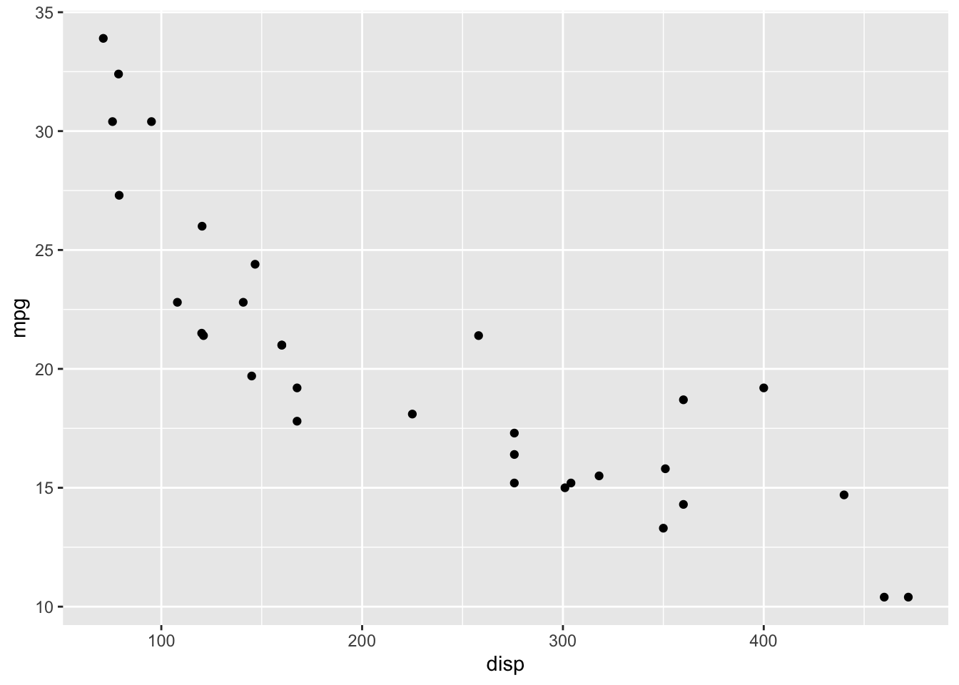
cor.test(mtcars$disp, mtcars$mpg, method='pearson')##
## Pearson's product-moment correlation
##
## data: mtcars$disp and mtcars$mpg
## t = -8.7472, df = 30, p-value = 9.38e-10
## alternative hypothesis: true correlation is not equal to 0
## 95 percent confidence interval:
## -0.9233594 -0.7081376
## sample estimates:
## cor
## -0.8475514There was a negative strong significant correlation (r = -.85) between disp and mpg. Are wt. and qsec correlated?
ggplot(mtcars, aes(x=wt, y=qsec)) +
  geom_point()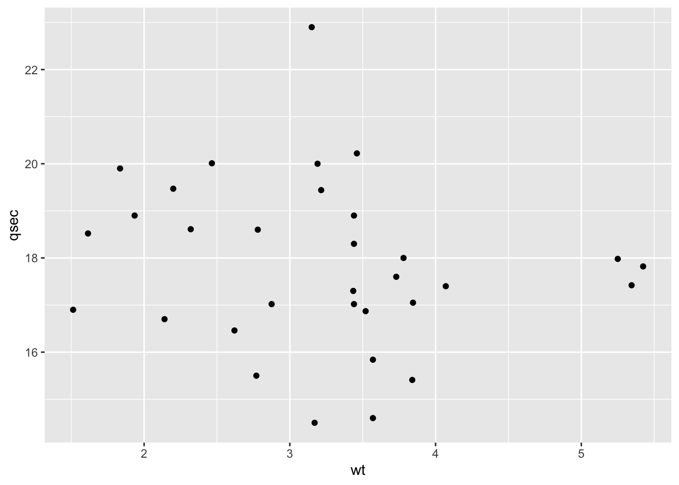
cor.test(mtcars$wt, mtcars$qsec, method='pearson')##
## Pearson's product-moment correlation
##
## data: mtcars$wt and mtcars$qsec
## t = -0.97191, df = 30, p-value = 0.3389
## alternative hypothesis: true correlation is not equal to 0
## 95 percent confidence interval:
## -0.4933536 0.1852649
## sample estimates:
## cor
## -0.1747159The p value is above .05 which indicates that we can retain the null hypothesis that there is no relationship between qsec and wt. Or as R puts it, the true correlation is equal to 0.
Kendall rank correlation coefficient can also be called for nonparametric correlation when the assumptions of a test (e.g. sample size, normality, etc.) are violated.
cor.test(x=mtcars$disp, y=mtcars$mpg, method='pearson')##
## Pearson's product-moment correlation
##
## data: mtcars$disp and mtcars$mpg
## t = -8.7472, df = 30, p-value = 9.38e-10
## alternative hypothesis: true correlation is not equal to 0
## 95 percent confidence interval:
## -0.9233594 -0.7081376
## sample estimates:
## cor
## -0.8475514cor.test(x=mtcars$disp, y=mtcars$mpg, method="kendall")## Warning in cor.test.default(x = mtcars$disp, y = mtcars$mpg, method =
## "kendall"): Cannot compute exact p-value with ties##
## Kendall's rank correlation tau
##
## data: mtcars$disp and mtcars$mpg
## z = -6.1083, p-value = 1.007e-09
## alternative hypothesis: true tau is not equal to 0
## sample estimates:
## tau
## -0.7681311Kendall’s rank correlation can be interpreted exactly the same as Pearson’s correlation coefficient in terms of magnitude and valence. Kendall’s estimates, however, are often more conservative than Pearson’s (tau = -.77, r = -.85). Judging by either test, there is a significant strong negative correlation between engine volume (disp) and miles per gallon (mpg).
4.3 Review
In this chapter we introduced descriptive statistics, concepts underlying normality, and some correlational methods. To make sure you understand this material, there is a practice assessment to go along with this and the next chapter at https://jayholster.shinyapps.io/StatsinRAssessment/
4.4 References
Revelle, W. (2017) psych: Procedures for Personality and Psychological Research, Northwestern University, Evanston, Illinois, USA, <https://CRAN.R-project.org/package=psych> Version = 1.7.8.
Wickham, H., Averick, M., Bryan, J., Chang, W., McGowan, L.D., François, R., Grolemund, G., Hayes, A., Henry, L., Hester, J., Kuhn, M., Pedersen, T.L., Miller, E., Bache, S.M., Müller, K., Ooms, J., Robinson, D., Seidel, D.P., Spinu, V., Takahashi, K., Vaughan, D., Wilke, C., Woo, K., & Yutani, H. (2019). Welcome to the tidyverse. Journal of Open Source Software, 4(43), 1686. https://doi.org/10.21105/joss.01686.
4.4.1 R Short Course Series
Video lectures of each guidebook chapter can be found at https://osf.io/6jb9t/. For this chapter, find the follow the folder path Statistics in R -> AY 2021-2022 Spring and access the video files, r markdown documents, and other materials for each short course.
4.4.2 Acknowledgements
This guidebook was created with support from the Center for Research Data and Digital Scholarship and the Laboratory for Interdisciplinary Statistical Analaysis at the University of Colorado Boulder, as well as the U.S. Agency for International Development under cooperative agreement #7200AA18CA00022. Individuals who contributed to materials related to this project include Jacob Holster, Eric Vance, Michael Ramsey, Nicholas Varberg, and Nickoal Eichmann-Kalwara.