Chapter 5 Exploring and Modeling Data
The purpose of this chapter is to expose you to several options for meaning-making with numbers beyond descriptive statistics. More specifically, you will be asked to apply your previous knowledge regarding descriptive statistics, data visualization, and data manipulation in the pursuit of the scientific method through statistical modeling.
Many interesting research questions are addressed with descriptive statistics. For instance, the census might ask the question: How many people live in the United States?relationships between and within variables tend to provide answers to more nuanced research questions—for instance, what is the relationship between median household income and educational attainment, or even what are the most influential predictors of happiness.
5.1 Quick Review
First, let’s review some of the things we’ve learned in this text so far. To get started, install and/or load the following packages into R Studio.
library(tidyverse)
library(SDT)
library(DataExplorer)
library(psych)
library(rstatix)
library(olsrr)
library(car)
We will be using a built-in dataset from the SDT package that contains
information on learning motivation data based on Self Determination
Theory. Call the dataset with the object name learning_motivation and
assign it to the object data with the operator <-. See the code
below.
To get a quick look at many facets of a dataset in one line of code, try
DataExplorer. DataExplorer includes an automated data exploration
process for analytic tasks and predictive modeling. Simply run the
function create_report() on a data frame to produce multiple plots and
tables related to descriptive and correlation related analyses. Use the
summary(), str(), and psych::describe() functions to examine and
assess the variables in the dataset for normality
For some more quick review, arrange the dataset by age in descending order. Then examine the first and last six rows of the dataset.
data <- data %>% arrange(desc(age))
head(data)
## sex age intrinsic identified introjected external
## 1 2 22 1.4 3.00 3.00 3.50
## 2 1 19 4.6 2.75 3.50 2.25
## 3 1 19 1.4 2.25 1.00 2.00
## 4 2 19 3.0 3.50 3.75 4.00
## 5 1 19 2.6 3.50 3.25 2.75
## 6 1 19 4.8 4.25 1.75 1.50tail(data)## sex age intrinsic identified introjected external
## 1145 2 10 3.6 4.75 3.50 4.25
## 1146 1 10 3.2 2.75 3.25 2.75
## 1147 1 10 3.6 4.25 3.00 3.50
## 1148 1 10 3.4 3.25 3.50 2.75
## 1149 2 10 3.2 3.00 3.25 2.75
## 1150 2 10 3.6 3.50 3.25 4.50Create a new column based on values from other columns without opening and saving the data file.
data <- data %>% mutate(internalizedmotivation = intrinsic + identified)
data <- data %>% mutate(internalizedmotivationlog = log10(intrinsic + identified))
head(data)
## sex age intrinsic identified introjected external internalizedmotivation
## 1 2 22 1.4 3.00 3.00 3.50 4.40
## 2 1 19 4.6 2.75 3.50 2.25 7.35
## 3 1 19 1.4 2.25 1.00 2.00 3.65
## 4 2 19 3.0 3.50 3.75 4.00 6.50
## 5 1 19 2.6 3.50 3.25 2.75 6.10
## 6 1 19 4.8 4.25 1.75 1.50 9.05
## internalizedmotivationlog
## 1 0.6434527
## 2 0.8662873
## 3 0.5622929
## 4 0.8129134
## 5 0.7853298
## 6 0.9566486psych::describe(data)## vars n mean sd median trimmed mad min max
## sex 1 1150 1.50 0.50 1.00 1.50 0.00 1.0 2
## age 2 1150 14.09 1.85 14.00 13.98 1.48 10.0 22
## intrinsic 3 1150 3.13 1.09 3.20 3.15 1.19 1.0 5
## identified 4 1150 3.29 1.01 3.25 3.34 1.11 1.0 5
## introjected 5 1150 2.75 1.04 2.75 2.73 1.11 1.0 5
## external 6 1150 2.94 0.94 3.00 2.95 1.11 1.0 5
## internalizedmotivation 7 1150 6.42 1.80 6.55 6.47 1.82 2.0 10
## internalizedmotivationlog 8 1150 0.79 0.14 0.82 0.80 0.12 0.3 1
## range skew kurtosis se
## sex 1.0 0.01 -2.00 0.01
## age 12.0 0.51 -0.04 0.05
## intrinsic 4.0 -0.15 -0.75 0.03
## identified 4.0 -0.39 -0.49 0.03
## introjected 4.0 0.12 -0.80 0.03
## external 4.0 -0.10 -0.49 0.03
## internalizedmotivation 8.0 -0.27 -0.39 0.05
## internalizedmotivationlog 0.7 -1.17 1.58 0.00Select rows of a data frame based on a certain condition. Use the
dim()function to ascertain the dimensions of the resultant dataset. If
1 represents males and 2 represents females, how many males are 18 or
older in the dataset?
malesover18 <- data %>% filter(age >= 18, sex == 1)
dim(malesover18)
## [1] 34 8Select specific columns of a data frame using the select() function.
Or select all columns except one using -column (e.g.
select(-intrinsic))
selected_data <- data %>% select(sex, age, intrinsic, external)
head(selected_data)
## sex age intrinsic external
## 1 2 22 1.4 3.50
## 2 1 19 4.6 2.25
## 3 1 19 1.4 2.00
## 4 2 19 3.0 4.00
## 5 1 19 2.6 2.75
## 6 1 19 4.8 1.50Use transformations as an opportunity to label your data categorically.
newdata <- data %>% mutate(preteen = age <= 12)
head(newdata)
## sex age intrinsic identified introjected external internalizedmotivation
## 1 2 22 1.4 3.00 3.00 3.50 4.40
## 2 1 19 4.6 2.75 3.50 2.25 7.35
## 3 1 19 1.4 2.25 1.00 2.00 3.65
## 4 2 19 3.0 3.50 3.75 4.00 6.50
## 5 1 19 2.6 3.50 3.25 2.75 6.10
## 6 1 19 4.8 4.25 1.75 1.50 9.05
## internalizedmotivationlog preteen
## 1 0.6434527 FALSE
## 2 0.8662873 FALSE
## 3 0.5622929 FALSE
## 4 0.8129134 FALSE
## 5 0.7853298 FALSE
## 6 0.9566486 FALSESave your edited data frame to a .csv file.
write_csv(data, "sdtedit.csv")5.2 Correlational Models
Next we will review and explore correlational models, which were conceptually covered in detail in the previous chapter. Most correlation coefficients are interpreted as a number between -1 and 1. This number tells us about the strength of the relationship between the two variables. Even if your final goal is regression or an inferential statistical test, correlations are useful to look at during exploratory data analysis before trying to fit a predictive model. Here are several correlation tasks using the Rstatix library.
# Correlation test between two variables
data %>% cor_test(age, intrinsic, method = "pearson")
## # A tibble: 1 × 8
## var1 var2 cor statistic p conf.low conf.high method
## <chr> <chr> <dbl> <dbl> <dbl> <dbl> <dbl> <chr>
## 1 age intrinsic -0.16 -5.61 0.0000000261 -0.219 -0.106 Pearson# Correlation of one variable against all
data %>% cor_test(intrinsic, method = "pearson")## # A tibble: 7 × 8
## var1 var2 cor statistic p conf.low conf.high method
## <chr> <chr> <dbl> <dbl> <dbl> <dbl> <dbl> <chr>
## 1 intrinsic sex 0.22 7.60 6.03e- 14 0.163 0.273 Pears…
## 2 intrinsic age -0.16 -5.61 2.61e- 8 -0.219 -0.106 Pears…
## 3 intrinsic identified 0.48 18.4 2.61e- 66 0.431 0.520 Pears…
## 4 intrinsic introjected 0.29 10.4 2.41e- 24 0.240 0.346 Pears…
## 5 intrinsic external -0.026 -0.881 3.78e- 1 -0.0837 0.0319 Pears…
## 6 intrinsic internalizedmo… 0.87 60.3 0 0.857 0.885 Pears…
## 7 intrinsic internalizedmo… 0.84 52.7 6.05e-309 0.824 0.857 Pears…# Pairwise correlation test between all variables
data %>% cor_test(method = "pearson")## # A tibble: 64 × 8
## var1 var2 cor statistic p conf.low conf.high method
## <chr> <chr> <dbl> <dbl> <dbl> <dbl> <dbl> <chr>
## 1 sex sex 1 Inf 0 1 1 Pears…
## 2 sex age 0.027 0.899 3.69e- 1 -0.0313 0.0842 Pears…
## 3 sex intrinsic 0.22 7.60 6.03e-14 0.163 0.273 Pears…
## 4 sex identified 0.13 4.60 4.62e- 6 0.0774 0.191 Pears…
## 5 sex introjected 0.039 1.33 1.82e- 1 -0.0185 0.0969 Pears…
## 6 sex external 0.0094 0.317 7.51e- 1 -0.0485 0.0671 Pears…
## 7 sex internalizedmotiva… 0.21 7.19 1.13e-12 0.152 0.262 Pears…
## 8 sex internalizedmotiva… 0.2 6.96 5.78e-12 0.145 0.256 Pears…
## 9 age sex 0.027 0.899 3.69e- 1 -0.0313 0.0842 Pears…
## 10 age age 1 Inf 0 1 1 Pears…
## # … with 54 more rows# Compute correlation matrix
cor.mat <- data %>% cor_mat()
cor.mat## # A tibble: 8 × 9
## rowname sex age intrinsic identified introjected external
## * <chr> <dbl> <dbl> <dbl> <dbl> <dbl> <dbl>
## 1 sex 1 0.027 0.22 0.13 0.039 0.0094
## 2 age 0.027 1 -0.16 -0.16 -0.13 -0.074
## 3 intrinsic 0.22 -0.16 1 0.48 0.29 -0.026
## 4 identified 0.13 -0.16 0.48 1 0.46 0.29
## 5 introjected 0.039 -0.13 0.29 0.46 1 0.5
## 6 external 0.0094 -0.074 -0.026 0.29 0.5 1
## 7 internalizedmotivation 0.21 -0.19 0.87 0.85 0.44 0.14
## 8 internalizedmotivatio… 0.2 -0.16 0.84 0.84 0.43 0.15
## # … with 2 more variables: internalizedmotivation <dbl>,
## # internalizedmotivationlog <dbl># Show the significance levels
cor.mat %>% cor_get_pval()## # A tibble: 8 × 9
## rowname sex age intrinsic identified introjected external
## <chr> <dbl> <dbl> <dbl> <dbl> <dbl> <dbl>
## 1 sex 0 3.69e- 1 6.03e- 14 4.62e- 6 1.82e- 1 7.51e- 1
## 2 age 3.69e- 1 0 2.61e- 8 2.16e- 8 5.05e- 6 1.2 e- 2
## 3 intrinsic 6.03e-14 2.61e- 8 0 2.61e- 66 2.41e-24 3.78e- 1
## 4 identified 4.62e- 6 2.16e- 8 2.61e- 66 0 1.26e-61 4.26e-23
## 5 introjected 1.82e- 1 5.05e- 6 2.41e- 24 1.26e- 61 0 1.03e-73
## 6 external 7.51e- 1 1.2 e- 2 3.78e- 1 4.26e- 23 1.03e-73 0
## 7 internalizedmotiv… 1.13e-12 7.54e-11 0 2.08e-316 2.47e-54 9.85e- 7
## 8 internalizedmotiv… 5.78e-12 3.57e- 8 6.05e-309 1.90e-300 6.78e-52 5.24e- 7
## # … with 2 more variables: internalizedmotivation <dbl>,
## # internalizedmotivationlog <dbl># Replacing correlation coefficients by symbols
cor.mat %>%
cor_as_symbols() %>%
pull_lower_triangle()## rowname sex age intrinsic identified introjected external
## 1 sex
## 2 age
## 3 intrinsic
## 4 identified .
## 5 introjected . .
## 6 external . .
## 7 internalizedmotivation * * .
## 8 internalizedmotivationlog * * .
## internalizedmotivation internalizedmotivationlog
## 1
## 2
## 3
## 4
## 5
## 6
## 7
## 8 *# Mark significant correlations
cor.mat %>%
cor_mark_significant()## rowname sex age intrinsic identified introjected
## 1 sex
## 2 age 0.027
## 3 intrinsic 0.22**** -0.16****
## 4 identified 0.13**** -0.16**** 0.48****
## 5 introjected 0.039 -0.13**** 0.29**** 0.46****
## 6 external 0.0094 -0.074* -0.026 0.29**** 0.5****
## 7 internalizedmotivation 0.21**** -0.19**** 0.87**** 0.85**** 0.44****
## 8 internalizedmotivationlog 0.2**** -0.16**** 0.84**** 0.84**** 0.43****
## external internalizedmotivation internalizedmotivationlog
## 1
## 2
## 3
## 4
## 5
## 6
## 7 0.14****
## 8 0.15**** 0.98****# Draw correlogram using R base plot
cor.mat %>%
cor_reorder() %>%
pull_lower_triangle() %>%
cor_plot()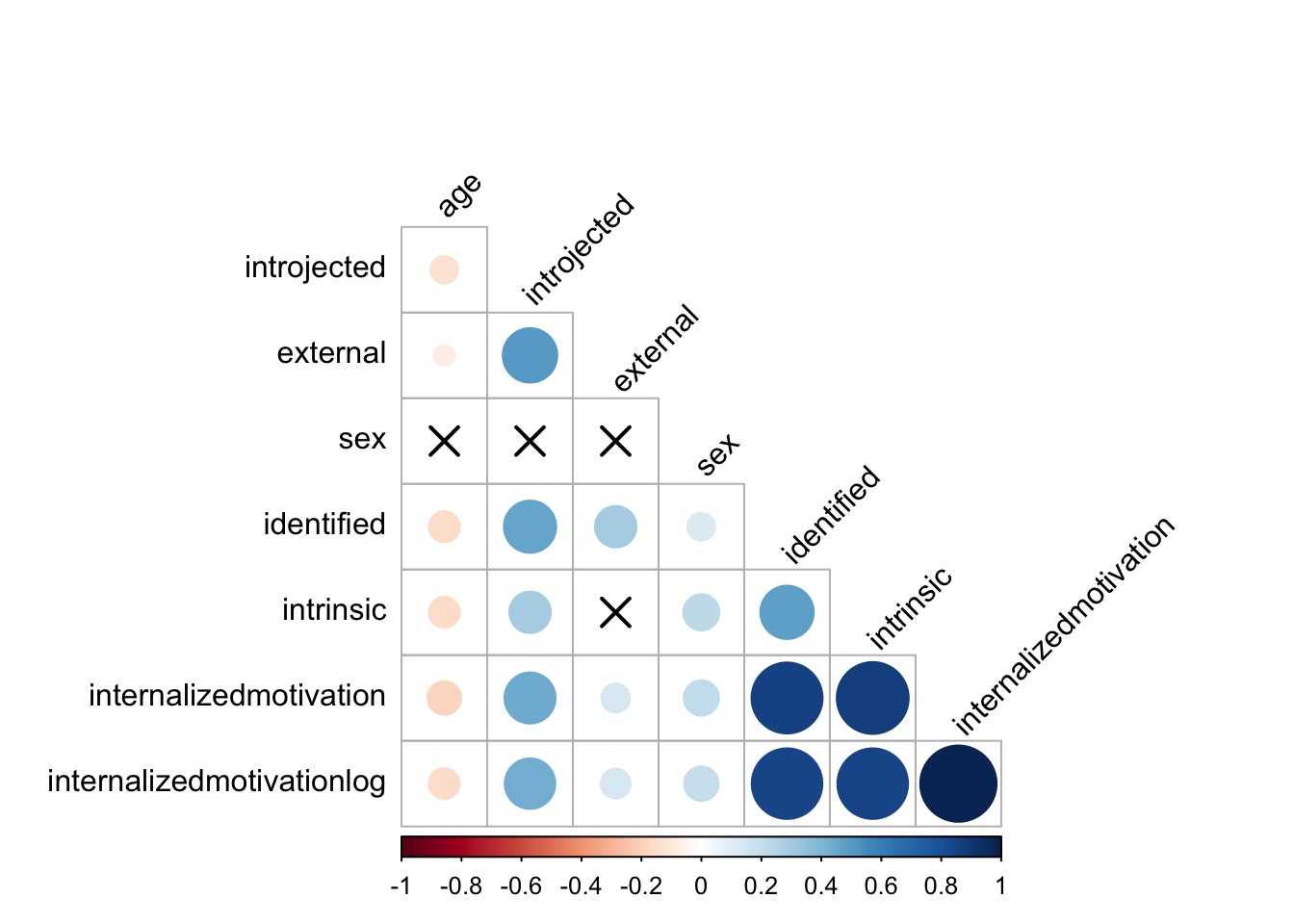
5.3 Simple and Multiple Regression
Researchers use either bivariate regression (simple—one dependent and one independent) or multiple regression (more than one independent and one dependent) as even more nuanced models of influence between two or more variables in a dataset. Dependent variables in each of these scenarios are often called criterion, outcome, or response variable, while the independent variable is often called the predictor or explanatory variable.
Regression is used to find relationships between variables—similarly to correlation analysis—however, there are three major differences between correlation and regression.
Test Purpose
“While correlation analyses are used to determine relationships and the strength of relationships between variables, researchers use regression analysis to predict, based on information from another variable or set of variables, the outcome of one variable. Otherwise, researchers can use regression analysis as a tool to explain why, based on any given predictor variables, differences exist between participants” (Russell, 2018, p. 193).
Variable Names
There must be a dependent variable in regression that a researcher is trying to predict based on other predictor (independent) variables. This concept is not used in correlation methods.
Regression Coefficients and Slope Intercepts
Researchers can use regression coefficients to infer beyond the direction and magnitude of relationships and discuss changes in Y due to specific changes in X (e.g., for every increase of 1 unit in Y, X increases .5)
The unstandardized regression formula is Y = a + bX where a is the
intercept (where the line of best fit crosses the y-axis) and b is the
slope of the regression line (½ is up 1 over 2). Put otherwise, a is
the value of Y when X = 0 and b is the regression coefficient. The null
hypothesis of the regression model is that independent variables are not
able to significantly predict the dependent variable (i.e., the slope or
standardized beta weight is 0, and that the predictor variable had no
impact on the dependent variable).
Here’s how you perform simple linear regression in R. This example uses the mtcars dataset which describes several measures of a set of cars. Let’s model quarter mile time (qsec) as predicted by horsepower then examine the intercepts and coefficients before visualizing the relationship in a scatter plot.
The following code represents the unstandardized regression formula
using the function lm() assigned to the object mod
mod <- lm(qsec ~ hp, data = mtcars)Use summary(mod) to display the statistical output. See the asterisks
for the level of significance, and the coefficient labelled ‘estimate’
as a description of the extent to which the target variable should
change as the predictor variable increases by 1 unit. The r-squared,
F-statistics, degrees of freedom, and p-value provide important model
fit and parsimony statistics that provide important context for the
interpretation of regression coefficients.
summary(mod)##
## Call:
## lm(formula = qsec ~ hp, data = mtcars)
##
## Residuals:
## Min 1Q Median 3Q Max
## -2.1766 -0.6975 0.0348 0.6520 4.0972
##
## Coefficients:
## Estimate Std. Error t value Pr(>|t|)
## (Intercept) 20.556354 0.542424 37.897 < 2e-16 ***
## hp -0.018458 0.003359 -5.495 5.77e-06 ***
## ---
## Signif. codes: 0 '***' 0.001 '**' 0.01 '*' 0.05 '.' 0.1 ' ' 1
##
## Residual standard error: 1.282 on 30 degrees of freedom
## Multiple R-squared: 0.5016, Adjusted R-squared: 0.485
## F-statistic: 30.19 on 1 and 30 DF, p-value: 5.766e-06It’s helpful to store the model coefficients as objects to be referred to in plotting procedures.
beta0 <- coef(mod)[1]
beta1 <- coef(mod)[2]
Use the geom_point() and geom_abline() functions to display a
scatterplot with a line of best fit.
ggplot(mtcars, aes(x = hp, y = qsec)) +
  geom_point() +
  geom_abline(intercept = beta0, slope = beta1, colour='red') +
  ggtitle("Quarter Mile Time as a function of Horsepower") +
  xlab('Horsepower') +
  ylab('Quarter Mile Time')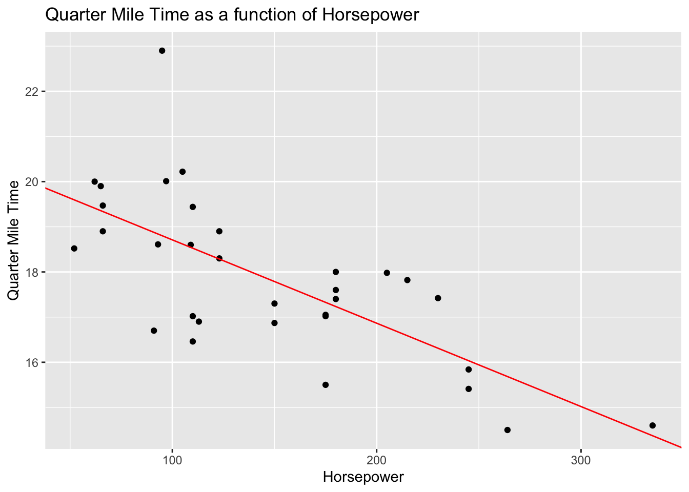
Practically, these findings suggest that horsepower is a significant predictor of quarter mile time. More specifically, the model output tells us that quarter mile time decreases by about 2 tenths of a second (.018) for each unit increase of horsepower in a given car. While statistically significant, this may seem practically insignificant. However, an increase of 100 horsepower tends to predict a loss of 1.8 seconds in quarter mile time, and a change in 300 horsepower tends to predict a loss of 5.4 seconds (which is good when the goal is speed). Is horsepower acting as a proxy for another variable? Put otherwise, would another variable (or set of variables) serve as better predictors of quarter mile time than hp?
Checking for Regression Assumptions
The assumptions of regression are as follows:
1. Linearity—relationship between dependent and independent variables is linear.
2. Homoscedasticity—the variance remains equal along the entire slope of the data
3. Normal distribution for variables included in the model.
4. Number of variables—rule of thumb is that you have 10-20 participants per variable. Others argue less works (5).
5. No multicollinearity—no two independent variables should be highly correlated as they would then be redundant in the model (no new information to interpret).
Let’s assess each of these assumptions for our model of quarter mile time as a function of horsepower.
Are the data linear? Use a quickplot to visually assess linearity.
plot(qsec ~ hp, data = mtcars, main = 'Quarter Mile time by Horsepower') # plots raw data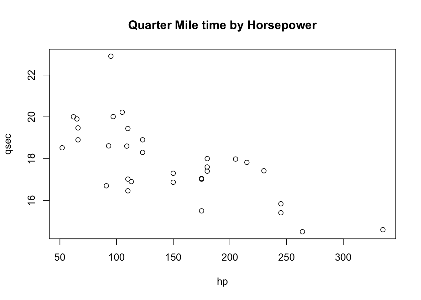
Are the data normally distributed? Use the plot() function to display
output relevant to several assumptions.
plot(mod)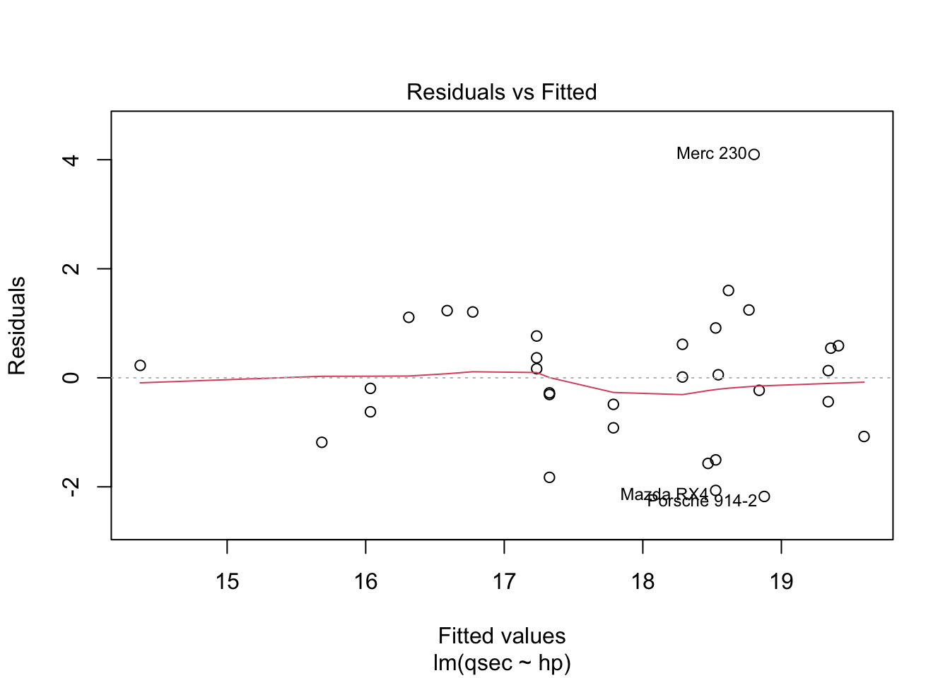
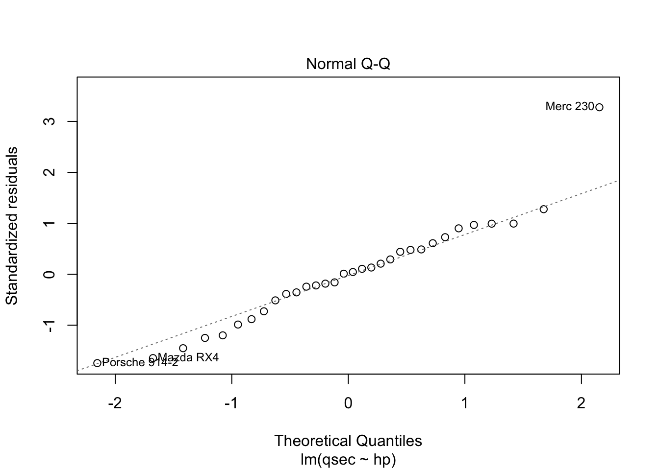
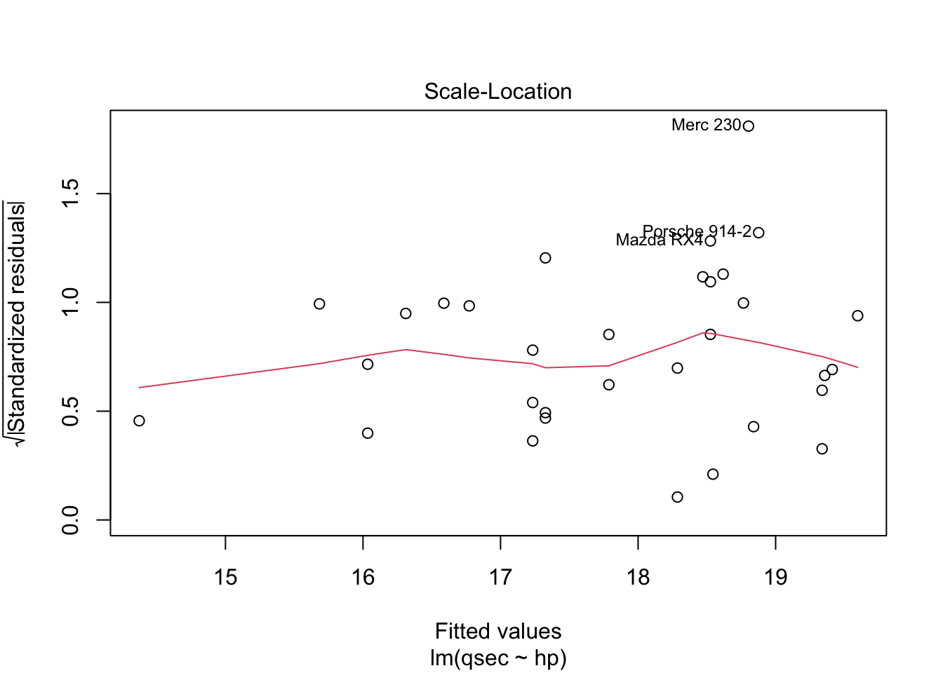
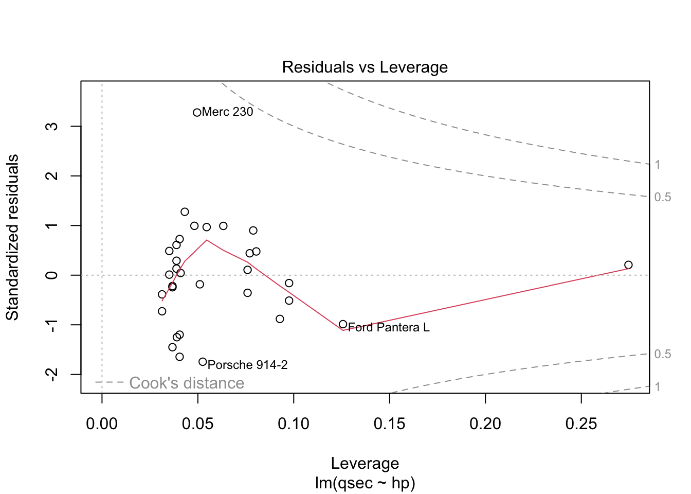
The residuals vs. fitted plot used to check linear relationship. A horizontal line without distinct patterns is an indication that the linear relationship is present. The normal Q-Q is used to examine whether residuals are normally distributed. If they are they will appear to be linear on this plot. The scale-location plot is used to check homogeneity of variance of residuals. A horizontal line with equally spread points is agood indication of homogeneity of variance. The residuals vs. leverage plot is used to identify potential outliers that are influencing regression results. The red lines are curves of constant Cook’s distance, another metric to determine the influence of a point which combines leverage and residual size.
You do not want to see a pattern to residuals when ordered by independent variable as “the assumption of homoscedasticity (meaning”same variance”) is central to linear regression models. Homoscedasticity describes a situation in which the error term (that is, the “noise” or random disturbance in the relationship between the independent variables and the dependent variable) is the same across all values of the independent variables. Heteroscedasticity (the violation of homoscedasticity) is present when the size of the error term differs across values of an independent variable. The impact of violating the assumption of homoscedasticity is a matter of degree, increasing as heteroscedasticity increases” (https://www.statisticssolutions.com/homoscedasticity/).
You can also check the multicollinearity assumption using variance
inflation factors with the command vif(). Variation inflation factors
greater than 5 or 10 (depending on the area of research) are often taken
as indicative that there may be a multicollinearity problem. This is
useful when constructing models with multiple predictor
variables—ensuring that two predictors are not too highly correlated
and predicting the same variance in the outcome variable.
mod <- lm(qsec ~ hp + cyl, data = mtcars)
vif(mod)
## GVIF Df GVIF^(1/(2*Df))
## hp 3.494957 1 1.869480
## cyl 3.494957 2 1.3672895.3.1 Multiple Regression
To estimate multiple regression equations, simply add additional predictors. This allows you to eliminate confounds and provide evidence for causality with your model (given sufficient internal/external validity and appropriate sampling procedures). In the example below, Quarter Mile Time is modeled as a function of horsepower and engine volume (disp). The adjusted r-squared value tells us that 51% of the variance in quarter mile time was explained by variance in horsepower.
mod2 <- lm(qsec ~ hp + disp, data = mtcars)
summary(mod2)
##
## Call:
## lm(formula = qsec ~ hp + disp, data = mtcars)
##
## Residuals:
## Min 1Q Median 3Q Max
## -2.0266 -0.9156 0.1675 0.6109 4.1752
##
## Coefficients:
## Estimate Std. Error t value Pr(>|t|)
## (Intercept) 20.454114 0.531156 38.509 < 2e-16 ***
## hp -0.025422 0.005339 -4.761 4.93e-05 ***
## disp 0.004870 0.002954 1.649 0.11
## ---
## Signif. codes: 0 '***' 0.001 '**' 0.01 '*' 0.05 '.' 0.1 ' ' 1
##
## Residual standard error: 1.247 on 29 degrees of freedom
## Multiple R-squared: 0.5443, Adjusted R-squared: 0.5129
## F-statistic: 17.32 on 2 and 29 DF, p-value: 1.124e-05Let’s model quarter mile time as a function of variance in mpg, number of cylinders, horsepower, and automatic/manual transmission.
mod2 <- lm(qsec ~ mpg + cyl + hp + am, data = mtcars)
summary(mod2)
##
## Call:
## lm(formula = qsec ~ mpg + cyl + hp + am, data = mtcars)
##
## Residuals:
## Min 1Q Median 3Q Max
## -1.7437 -0.6751 0.1015 0.5319 2.1426
##
## Coefficients:
## Estimate Std. Error t value Pr(>|t|)
## (Intercept) 20.426987 1.772405 11.525 1.02e-11 ***
## mpg -0.012876 0.066295 -0.194 0.847512
## cyl.L -1.951811 0.631743 -3.090 0.004730 **
## cyl.Q 0.173954 0.358954 0.485 0.632009
## hp -0.008707 0.005815 -1.497 0.146337
## ammanual -2.307268 0.513173 -4.496 0.000127 ***
## ---
## Signif. codes: 0 '***' 0.001 '**' 0.01 '*' 0.05 '.' 0.1 ' ' 1
##
## Residual standard error: 0.931 on 26 degrees of freedom
## Multiple R-squared: 0.7724, Adjusted R-squared: 0.7286
## F-statistic: 17.64 on 5 and 26 DF, p-value: 1.249e-07This model seems to indicate that the number of cylinders and type of transmission (am) are the strongest predictors of quarter mile time (-2.37 seconds per change in transmission type, and -0.70 seconds per change in cylinders). These variables collectively account for a larger portion of variance given the adjusted r-squared (used with multiple variables) of .74.
We can also use the olsrr library to run stepwise regression and
identify the best fitting model. Insert a period instead of variables to
call all variables in the dataset.
model <- lm(qsec ~ ., data = mtcars)
modelchoice <- ols_step_all_possible(model) %>% arrange(desc(adjr)) %>% filter(n <= 4)
head(modelchoice)
## Index N Predictors R-Square Adj. R-Square Mallow's Cp
## 1 177 4 hp wt gear wtqsec_ratio 0.9735351 0.9684457 12.20563
## 2 176 4 cyl wt carb wtqsec_ratio 0.9750342 0.9648209 10.26807
## 3 180 4 mpg hp wt wtqsec_ratio 0.9661794 0.9611690 21.71273
## 4 179 4 cyl hp wt wtqsec_ratio 0.9669874 0.9606388 20.66849
## 5 182 4 hp wt vs wtqsec_ratio 0.9648571 0.9596508 23.42181
## 6 56 3 hp wt wtqsec_ratio 0.9635221 0.9596137 23.14730model2 <- lm(qsec ~ disp + wt + vs + carb, data=mtcars)
summary(model2)##
## Call:
## lm(formula = qsec ~ disp + wt + vs + carb, data = mtcars)
##
## Residuals:
## Min 1Q Median 3Q Max
## -1.25620 -0.51160 -0.05549 0.37667 2.53603
##
## Coefficients:
## Estimate Std. Error t value Pr(>|t|)
## (Intercept) 13.000767 0.734959 17.689 6.90e-15 ***
## disp -0.013590 0.003696 -3.677 0.001249 **
## wt 2.099573 0.399921 5.250 2.51e-05 ***
## vsstraight 1.319133 0.588394 2.242 0.034906 *
## carb.L -3.180956 0.697400 -4.561 0.000139 ***
## carb.Q -0.022039 0.586603 -0.038 0.970355
## carb.C 0.243124 0.571370 0.426 0.674420
## carb^4 0.006197 0.563858 0.011 0.991327
## carb^5 0.246119 0.495808 0.496 0.624323
## ---
## Signif. codes: 0 '***' 0.001 '**' 0.01 '*' 0.05 '.' 0.1 ' ' 1
##
## Residual standard error: 0.7901 on 23 degrees of freedom
## Multiple R-squared: 0.8549, Adjusted R-squared: 0.8045
## F-statistic: 16.95 on 8 and 23 DF, p-value: 6.049e-08After searching for the best model with the fewest number of predictors, it can be determined that displacement, weight, engine style (v shaped vs. straight) and carb explain the 82%, the same amount of variance in quarter mile time as the entire dataset explains.
plot(residuals(mod2))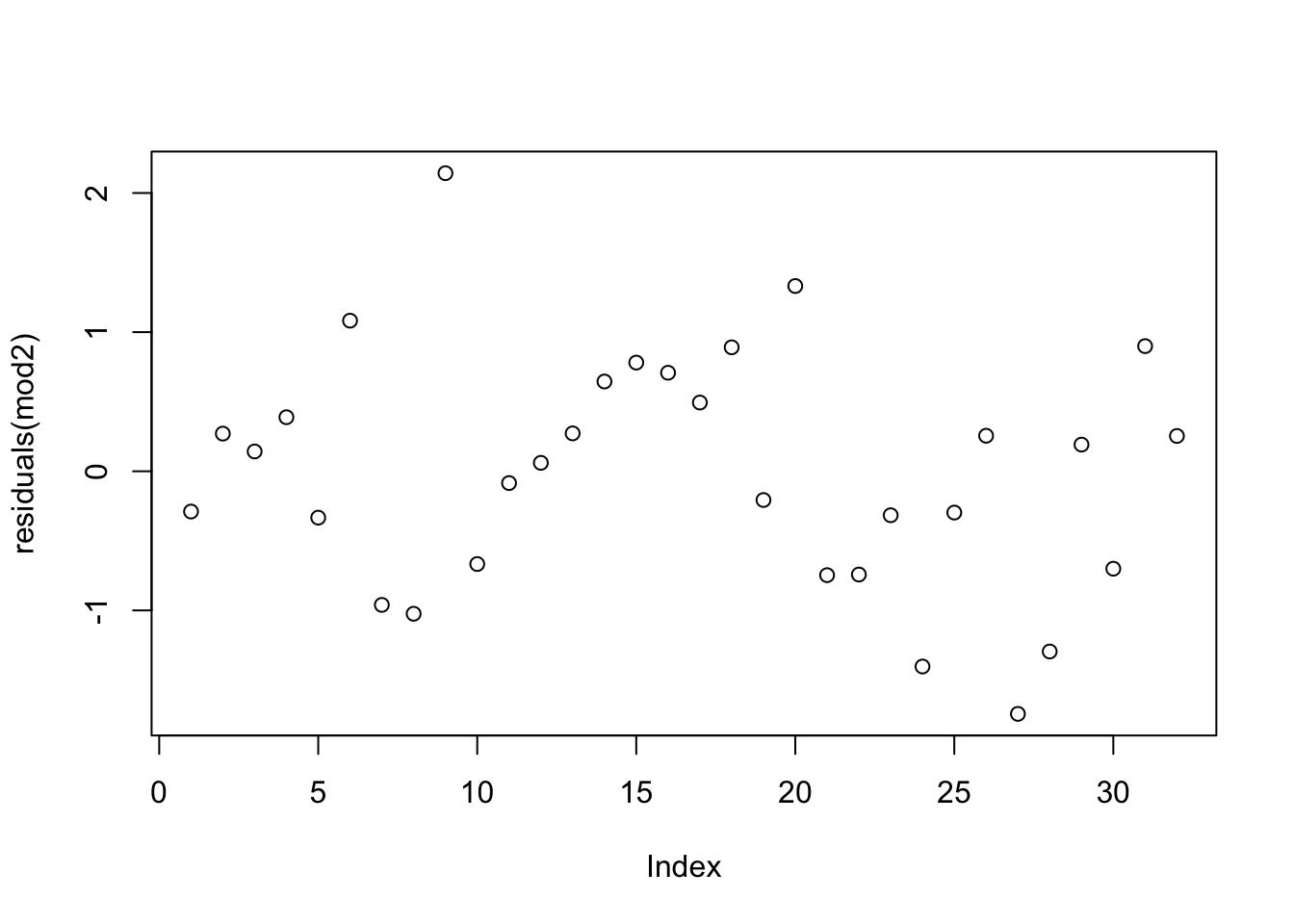
You can store the elements of the summary such as r-squared.
summ_mod <- summary(mod)
summ_mod$residuals
summ_mod$r.squared
summ_mod$adj.r.squared
summ_mod$coefficients
Generalized linear models are fairly common. Logistic regression is used
when the response variable is binary, e.g., did you vote (yes or no), do
you have a diabetes (yes or no). Poisson regression is used when the
response variable is a count (i.e., numeric but not continuous, e.g.,
how many heart attacks have you had, how many days from outbreak to
infection). Fitting such models in R is very similar to how one would
fit a linear model. E.g., for poisson regression,
glm(counts ~ outcome + treatment, data, family = poisson()).
5.4 Inferential Statistics
5.4.1 Hypothesis Testing
A hypothesis is a proposed solution to a problem. Hypothesis testing is a means to take a rational (logical) decision based on observed data In music education, hypotheses tend to have an underlying goal of increased student success* (What can success mean here?) After formulating some hypothesis (e.g., there is no difference in performance ability between 6th and 7th grade band students), we collect and use data to accept or reject the hypothesis (null in this case).
A null hypothesis \(H_0\): a statement that represents the phenomenon you may want to provide evidence against (e.g., two means are the same where group difference is expected). An alternative hypothesis \(H_1\): represents the opposite of the null hypothesis (e.g., two group means are statistically different).
For example, if you want to test whether automatic/manual transmission affect miles per gallon (mpg), then \(H_0\) would be that manual and automatic transmission cars have the same mpg and \(H_1\) would be that manual and automatic transmission cars have different mpg.
5.4.2 The Role of Statistics in Hypothesis Testing
Statistical tests are designed to reject or not reject a null hypothesis based on data. They do not allow you to find evidence for the alternative; just evidence for/against the null hypothesis. Assuming that \(H_0\) is true, the p-value for a test is the probability of observing data as extreme or more extreme than what you actually observed (i.e., how surprised should I be about this?).
The significance level \(\alpha\) is what you decide this probability should be (i.e., the surprise threshold that you will allow), that is, the probability of a Type I error (rejecting \(H_0\) when it is true). Oftentimes, \(\alpha = 5\% = 0.05\) is accepted although much lower alpha values are common in some research communities, and higher values are used for exploratory research in less defined fields. If we set \(\alpha = 0.05\), we reject \(H_0\) if p-value < 0.05 and say that we have found evidence against \(H_0\).
Note that statistical tests and methods usually have assumptions about the data and the model. The accuracy of the analysis and the conclusions derived from an analysis depend crucially on the validity of these assumptions. So, it is important to know what those assumptions are and to determine whether they hold.
5.4.3 Checking Biases
Biases are in reference to preconceived notions about how something does or does not work, an opinion you hold about how something should work, and your understanding of how the world operates. Positivism is an episitomological belief that the knowledge serves only to describe what we observe. However, we, the observer, are entrenched in known and unknown biases. In the view of the positivist, the world is deterministic, and can be modeled and understood in complete objectivity. As positivism does not account for our biases, social scientists shifted to a post-positivist view. Post-positivism holds space for our biases through the acknowledgement that scientific reasoning and our acquired sense of the world are not the same. Most importantly, this epistemological view allows for the revision of theory, and holds that the goal of science is to describe reality in the most accurate way possible, understanding that we can never achieve that goal.
5.4.4 Tests of Group Differences
Before testing whether means are different among groups, it can be helpful to visualize the data distribution.
ggplot(mtcars) +
geom_boxplot(aes(x=am, y=mpg)) 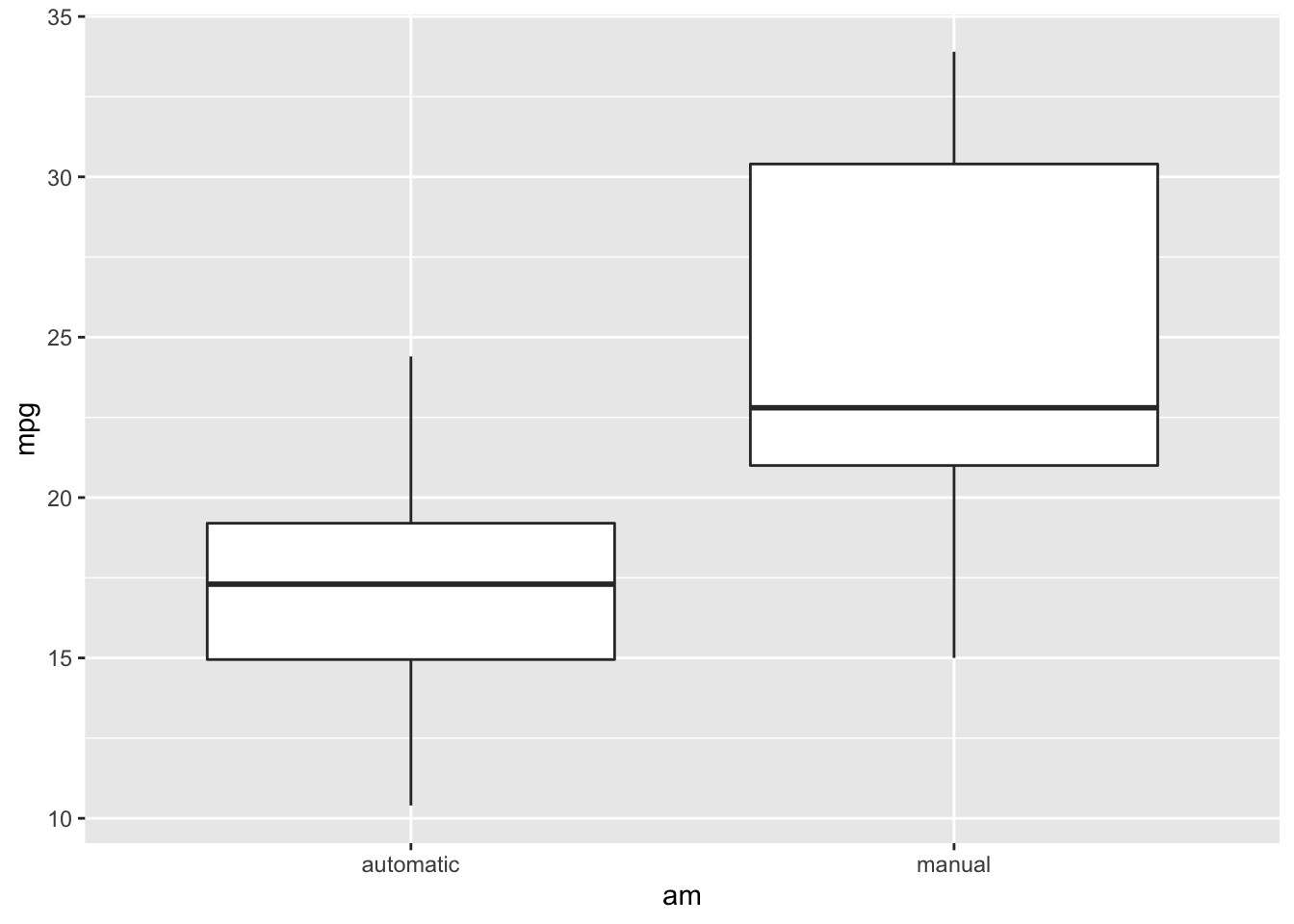
Remember, violin plots are similar to box plots except that violin plots show the probability density of the data at different values.
ggplot(mtcars) +
  geom_violin(aes(x = am, y = mpg, fill = am))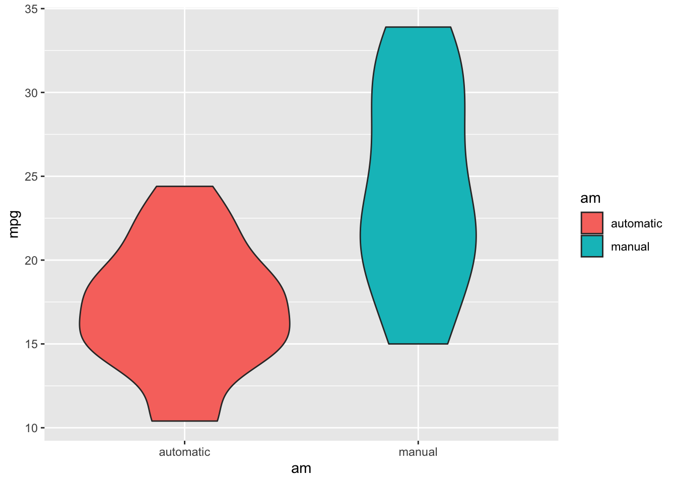
T-tests can be used to test whether the means of two groups are significantly different. The null hypothesis \(H_0\) assumes that the true difference in means \(\mu_d\) is equal to zero. The alternative hypothesis can be that \(\mu_d \neq 0\), \(\mu_d >0\), or \(\mu_d<0\). By default, the alternative hypothesis is that \(\mu_d \neq 0\).
t.test(mtcars$mpg ~ mtcars$am, alternative="two.sided")##
## Welch Two Sample t-test
##
## data: mtcars$mpg by mtcars$am
## t = -3.7671, df = 18.332, p-value = 0.001374
## alternative hypothesis: true difference in means between group automatic and group manual is not equal to 0
## 95 percent confidence interval:
## -11.280194 -3.209684
## sample estimates:
## mean in group automatic mean in group manual
## 17.14737 24.39231library(webr)## Registered S3 method overwritten by 'ggforce':
## method from
## scale_type.units unitsmodel <- t.test(mtcars$mpg ~ mtcars$am, alternative = "less")
plot(model)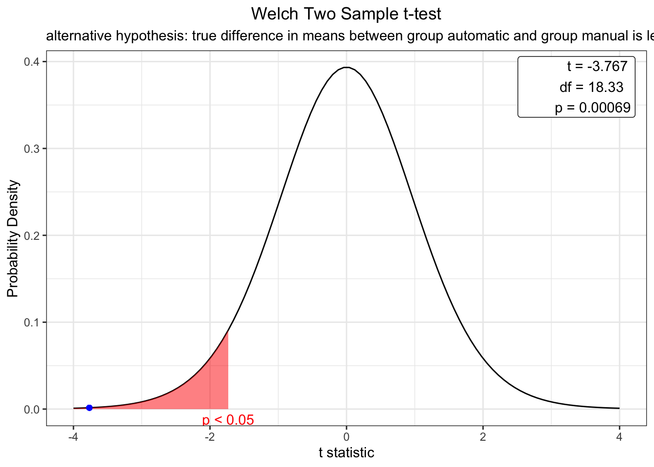
The t test results indicate that there is a significant difference in mpg between cars with a manual (0) and automatic (0) transmission (t = -3.77, p < .001). The webr library also allows you to easily produce distribution plots. Using this plot, we can determine that the null hypothesis will only be true (no difference between mpg by transmission type) < .01% of the time. Most differences are significant (p < .05) when t values exceed +- 1.96.
T-tests require a normality assumption which may or may not be valid
depending on the situation. The function wilcox.test allows us compare
group medians (not means) in a non-parametric setting (i.e., without the
assumption of the data coming from some probability distribution). You
may have heard of the Mann-Whitney U test. This test is just a
two-sample Wilcoxon test. Is the median mpg different for automatic and
manual cars?
wilcox.test(mtcars$mpg ~ mtcars$am)##
## Wilcoxon rank sum test with continuity correction
##
## data: mtcars$mpg by mtcars$am
## W = 42, p-value = 0.001871
## alternative hypothesis: true location shift is not equal to 0Yes, there is a significant difference in the median of mpg across transmission types (W = 42, p = .002)
5.4.5 Reporting Support
Writing up statistical reports are a vital skill for researchers. The report library supports automated APA compliant reports for statistical analyses. For instance, the previous t-test is assigned to an object, and that object is passed through the “report()” function. The output includes all the important facets for reporting a t-test—including confidence intervals, a t-value, degrees of freedom, a p-value, and Cohen’s d (i.e., a reflection of the mean difference between groups in terms of standard deviations).
library(report)
ttestoutcome <- t.test(mtcars$mpg ~ mtcars$am, alternative="two.sided")
report(ttestoutcome)
## Effect sizes were labelled following Cohen's (1988) recommendations.
##
## The Welch Two Sample t-test testing the difference of mtcars$mpg by mtcars$am (mean in group automatic = 17.15, mean in group manual = 24.39) suggests that the effect is negative, statistically significant, and large (difference = -7.24, 95% CI [-11.28, -3.21], t(18.33) = -3.77, p = 0.001; Cohen's d = -1.41, 95% CI [-2.26, -0.53])5.4.6 Inferential Modeling
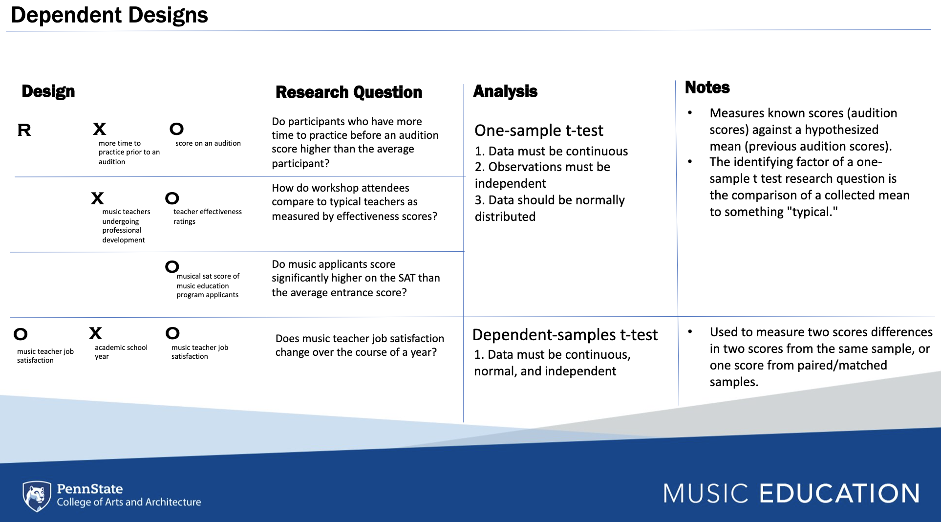
In this section, each chunk will include the code for running an
univariate method of statistical analysis in baseR and other
libraries. The figure below describes four separate dependent designs
that are associated with two basic inferential models which can be
analyzed using a one-sample t-test, where a mean with an unknown
distribution (e.g., M = 48) is assessed against a known distribution
of data. The dependent samples t-test is used to measure score
differences from paired or matched samples.
5.4.6.1 One Sample T-Test
We’re going to use the band participation dataset for these examples.
For the one sample t-test, call in the vector where your data are loaded
from, and use the argument mu to define the previously known mean
(with an unknown distribution). Examine both the output of the
statistical test and the automated written report.
data <- read_csv('participationdata.csv')
data <- data %>% drop_na(GradeLevel)

t.test(data$intentionscomp, mu = 5)
##
## One Sample t-test
##
## data: data$intentionscomp
## t = 9.5182, df = 39, p-value = 1.017e-11
## alternative hypothesis: true mean is not equal to 5
## 95 percent confidence interval:
## 11.18181 14.51819
## sample estimates:
## mean of x
## 12.85onesamplewriteup <- t.test(data$intentionscomp, mu = 5)
report(onesamplewriteup)## Effect sizes were labelled following Cohen's (1988) recommendations.
##
## The One Sample t-test testing the difference between data$intentionscomp (mean = 12.85) and mu = 5 suggests that the effect is positive, statistically significant, and large (difference = 7.85, 95% CI [11.18, 14.52], t(39) = 9.52, p < .001; Cohen's d = 1.50, 95% CI [1.06, 1.98])5.4.6.2 Dependent Sample T-Test
To run a dependent sample t-test, use the argument paired = TRUE
t.test(data$Intentions1, data$Intentions2, paired = TRUE)##
## Paired t-test
##
## data: data$Intentions1 and data$Intentions2
## t = 0.1383, df = 39, p-value = 0.8907
## alternative hypothesis: true mean difference is not equal to 0
## 95 percent confidence interval:
## -0.3406334 0.3906334
## sample estimates:
## mean difference
## 0.025dependentsamplewriteup <- t.test(data$Intentions1, data$Intentions2, paired = TRUE)
report(dependentsamplewriteup)## Effect sizes were labelled following Cohen's (1988) recommendations.
##
## The Paired t-test testing the difference between data$Intentions1 and data$Intentions2 (mean difference = 0.03) suggests that the effect is positive, statistically not significant, and very small (difference = 0.03, 95% CI [-0.34, 0.39], t(39) = 0.14, p = 0.891; Cohen's d = 0.02, 95% CI [-0.29, 0.34])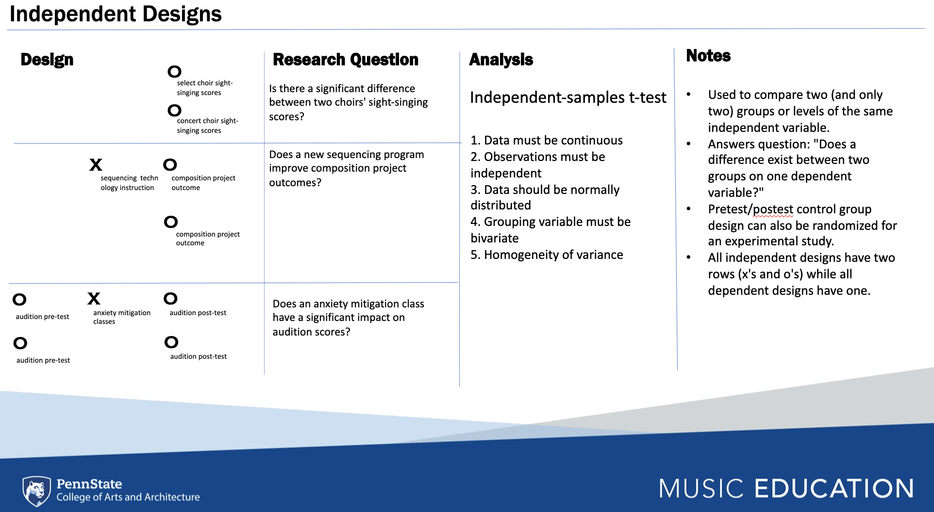
Independent designs are used to compare a measures across differing samples, whereas dependent designs assess differences within a sample.
5.4.6.3 Independent Samples T-Test
Here is another chance to run a basic t-test
t.test(data$intentionscomp ~ data$GradeLevel, var.equal = T)##
## Two Sample t-test
##
## data: data$intentionscomp by data$GradeLevel
## t = -2.9009, df = 38, p-value = 0.006156
## alternative hypothesis: true difference in means between group eighth-grade and group seventh-grade is not equal to 0
## 95 percent confidence interval:
## -8.125373 -1.446055
## sample estimates:
## mean in group eighth-grade mean in group seventh-grade
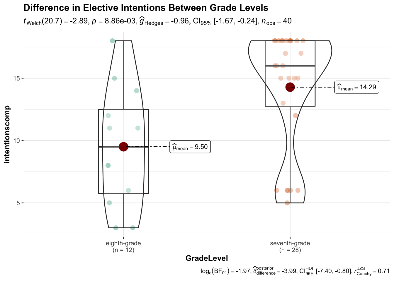
## 9.50000 14.28571Let’s try plotting the difference using ggstatsplot.
library(ggstatsplot)

ggbetweenstats(
  data = data,
  x = GradeLevel,
  y = intentionscomp,
  title = "Difference in Elective Intentions Between Grade Levels"
)
And for the write up?
ttestwriteup <- t.test(data$intentionscomp ~ data$GradeLevel, var.equal = T)
report(ttestwriteup)
## Effect sizes were labelled following Cohen's (1988) recommendations.
##
## The Two Sample t-test testing the difference of data$intentionscomp by data$GradeLevel (mean in group eighth-grade = 9.50, mean in group seventh-grade = 14.29) suggests that the effect is negative, statistically significant, and large (difference = -4.79, 95% CI [-8.13, -1.45], t(38) = -2.90, p = 0.006; Cohen's d = -1.00, 95% CI [-1.71, -0.28])5.4.6.4 One-Way ANOVA
There are multiple new terms that emerge when discussing ANOVA approaches. These include:
Within-subjects factors: the task(s) all participants did (i.e., repeated measures)
Between-subjects factors: separate groups did certain conditions (e.g., levels of an experimental variable)
Mixed design: differences were assessed for variables by participants (within-subjects), and something separates them into groups (e.g., between-subjects)
A main effect is the overall effect of a variable on particular groups.
Sometimes you have more than one IV, so you might have two main effects: one for Variable 1 and one for Variable 2.
Also, you can have an interaction between the variables such that performance in “cells” of data is affected variably by the other variable. You can report a significant p-value for the interaction line IF there is a significant main effect p-value.
You can only report a significant interaction if there is a significant main effect.
Interpreting the main effect doesn’t make sense: interpreting the interaction DOES (e.g., the main effect changes based on membership in one of the groups)
One-way ANOVAs are like t-tests, but they compare differences across
more than two groups (i.e., categorical variables. For instance, in the
participation dataset, you might compare socioeconomic status across the
four schools contributing students to the sample. To run the ANOVA,
first assign the model using the function aov() with the continuous
comparison variable (e.g., SES and the categorical vector of comparison
(e.g., School). To see the statistical output, run the summary()
function with the model name inside the parenthesis.
model <- aov(SESComp ~ data$School, data = data)
summary(model)
## Df Sum Sq Mean Sq F value Pr(>F)
## data$School 3 2.804 0.9345 7.881 4e-04 ***
## Residuals 34 4.032 0.1186
## ---
## Signif. codes: 0 '***' 0.001 '**' 0.01 '*' 0.05 '.' 0.1 ' ' 1
## 2 observations deleted due to missingnessThe output reflected a significant difference is present among the four schools. However, it is not possible to determine which schools are significantly different from others without Tukey’s HSD, which allows you to examine mean differences between each combination of school. Note the school relationships with a p value below .05 to see what schools differ statistically.
TukeyHSD(model)## Tukey multiple comparisons of means
## 95% family-wise confidence level
##
## Fit: aov(formula = SESComp ~ data$School, data = data)
##
## $`data$School`
## diff lwr upr p adj
## School2-School1 0.6673611 0.2721651 1.06255711 0.0003541
## School3-School1 0.2377315 -0.2141924 0.68965540 0.4955172
## School4-School1 0.3895833 -0.2400647 1.01923134 0.3542291
## School3-School2 -0.4296296 -0.8093217 -0.04993759 0.0215282
## School4-School2 -0.2777778 -0.8577669 0.30221139 0.5732634
## School4-School3 0.1518519 -0.4681826 0.77188635 0.9107596The reporting function produces information regarding the main effect in the model. For more on how to report Tukey’s HSD, visit https://statistics.laerd.com/spss-tutorials/one-way-anova-using-spss-statistics-2.php
report(model)## For one-way between subjects designs, partial eta squared is equivalent to eta squared.
## Returning eta squared.## Warning: 'data_findcols()' is deprecated and will be removed in a future update.
## Its usage is discouraged. Please use 'data_find()' instead.## Warning: Using `$` in model formulas can produce unexpected results. Specify your
## model using the `data` argument instead.
## Try: SESComp ~ School, data =
## data## The ANOVA (formula: SESComp ~ data$School) suggests that:
##
## - The main effect of data$School is statistically significant and large (F(3, 34) = 7.88, p < .001; Eta2 = 0.41, 95% CI [0.17, 1.00])
##
## Effect sizes were labelled following Field's (2013) recommendations.Factorial/Two-Way ANOVA
For factorial ANOVAs, there should be more than one categorical independent variable with one dependent variable (more dependent variables should be MANOVA) You are assessing first for main effects (between groups) and then for interaction effects (within groups)
Factorial ANOVAs are named more specifically for their number groupings Some examples are listed below:
2 x 2 x 2 ANOVA = Three independent variables with two levels each (e.g., gender, certified to teach or not, instrumentalist or not—main effects and interaction effects)
2 x 3 x 4 ANOVA = three independent variables, one has two levels (certified or not), one has three levels (teach in a rural, suburban, or urban school) and one has four levels (no music ed degree, music ed bachelors, music ed masters, music ed doctorate)
2 x 3 = two independent variables each one with two levels (gender) another with three levels (degree type)
To conduct a factorial ANOVA in R, use an asterisk to connect the two categorical variables of interest, as seen below. Then, use the summary function, Tukey HSD, and report function to interpret the output.
factorial <- aov(intentionscomp ~ Class*GradeLevel, data = data)
summary(factorial)
## Df Sum Sq Mean Sq F value Pr(>F)
## Class 1 16.6 16.55 0.701 0.40783
## GradeLevel 1 178.1 178.14 7.548 0.00932 **
## Class:GradeLevel 1 16.8 16.82 0.713 0.40415
## Residuals 36 849.6 23.60
## ---
## Signif. codes: 0 '***' 0.001 '**' 0.01 '*' 0.05 '.' 0.1 ' ' 1TukeyHSD(factorial)## Tukey multiple comparisons of means
## 95% family-wise confidence level
##
## Fit: aov(formula = intentionscomp ~ Class * GradeLevel, data = data)
##
## $Class
## diff lwr upr p adj
## orchestra-band 1.288221 -1.831278 4.40772 0.4078281
##
## $GradeLevel
## diff lwr upr p adj
## seventh-grade-eighth-grade 4.525003 1.125608 7.924398 0.0105076
##
## $`Class:GradeLevel`
## diff lwr upr
## orchestra:eighth-grade-band:eighth-grade 2.6250000 -5.38701652 10.637017
## band:seventh-grade-band:eighth-grade 5.8365385 -0.04267434 11.715751
## orchestra:seventh-grade-band:eighth-grade 5.5083333 -0.21962035 11.236287
## band:seventh-grade-orchestra:eighth-grade 3.2115385 -4.26927785 10.692355
## orchestra:seventh-grade-orchestra:eighth-grade 2.8833333 -4.47920176 10.245868
## orchestra:seventh-grade-band:seventh-grade -0.3282051 -5.28599268 4.629582
## p adj
## orchestra:eighth-grade-band:eighth-grade 0.8139391
## band:seventh-grade-band:eighth-grade 0.0522852
## orchestra:seventh-grade-band:eighth-grade 0.0631394
## band:seventh-grade-orchestra:eighth-grade 0.6577297
## orchestra:seventh-grade-orchestra:eighth-grade 0.7187103
## orchestra:seventh-grade-band:seventh-grade 0.9979489report(factorial)## Warning: 'data_findcols()' is deprecated and will be removed in a future update.
## Its usage is discouraged. Please use 'data_find()' instead.## The ANOVA (formula: intentionscomp ~ Class * GradeLevel) suggests that:
##
## - The main effect of Class is statistically not significant and small (F(1, 36) = 0.70, p = 0.408; Eta2 (partial) = 0.02, 95% CI [0.00, 1.00])
## - The main effect of GradeLevel is statistically significant and large (F(1, 36) = 7.55, p = 0.009; Eta2 (partial) = 0.17, 95% CI [0.03, 1.00])
## - The interaction between Class and GradeLevel is statistically not significant and small (F(1, 36) = 0.71, p = 0.404; Eta2 (partial) = 0.02, 95% CI [0.00, 1.00])
##
## Effect sizes were labelled following Field's (2013) recommendations.The more complex a model is the larger the sample size needs to be. As such, the lack of a significant effect may be due to low study power rather than the lack of the phenomenon of interest.
The MANOVA is an extended technique which determines the effects of independent categorical variables on multiple continuous dependent variables. It is usually used to compare several groups with respect to multiple continuous variables.
5.4.6.5 ANCOVA
The Analysis of Covariance (ANCOVA) is used in examining the differences in the mean values of the dependent variables that are related to the effect of the controlled independent variables while taking into account the influence of the uncontrolled independent variables as covariates. Use an addition operator to add covariates to the model.
ancova_model <- aov(intentionscomp ~ GradeLevel + valuescomp, data = data)
summary(ancova_model, type="III")
## Df Sum Sq Mean Sq F value Pr(>F)
## GradeLevel 1 178.9 178.92 9.73 0.00362 **
## valuescomp 1 208.4 208.37 11.33 0.00186 **
## Residuals 35 643.6 18.39
## ---
## Signif. codes: 0 '***' 0.001 '**' 0.01 '*' 0.05 '.' 0.1 ' ' 1
## 2 observations deleted due to missingnessreport(ancova_model)## Warning: 'data_findcols()' is deprecated and will be removed in a future update.
## Its usage is discouraged. Please use 'data_find()' instead.## The ANOVA (formula: intentionscomp ~ GradeLevel + valuescomp) suggests that:
##
## - The main effect of GradeLevel is statistically significant and large (F(1, 35) = 9.73, p = 0.004; Eta2 (partial) = 0.22, 95% CI [0.05, 1.00])
## - The main effect of valuescomp is statistically significant and large (F(1, 35) = 11.33, p = 0.002; Eta2 (partial) = 0.24, 95% CI [0.07, 1.00])
##
## Effect sizes were labelled following Field's (2013) recommendations.5.5 Review
In this chapter we reviewed necessary skills for successful R coding, in addition to introducing correlational and inferential statistical modeling procedures. To make sure you understand this material, there is a practice assessment to go along with this and the previous chapter at https://jayholster.shinyapps.io/StatsinRAssessment/
5.6 References
Cui B., (2020). DataExplorer. https://cran.r-project.org/web/packages/DataExplorer/index.html
Fox, J., & Weisberg, S. (2019). An R Companion to Applied Regression, Third edition. Sage, Thousand Oaks CA. https://socialsciences.mcmaster.ca/jfox/Books/Companion/.
Kassambara, A. (2021). Rstatix. https://cran.r-project.org/web/packages/rstatix/index.html
Hebbali, A. (2020). olsrr. https://cran.r-project.org/web/packages/olsrr/index.html
Makowski, D., Lüdecke, D., Mattan S., Patil, I., Wiernik, B. M., & Siegel, R. (2022). report: Automated Reporting of Results and Statistical Models. https://cran.r-project.org/web/packages/report/index.html
Revelle, W. (2017) psych: Procedures for Personality and Psychological Research, Northwestern University, Evanston, Illinois, USA, <https://CRAN.R-project.org/package=psych> Version = 1.7.8.
Russell, J. A. (2018). Statistics in music education research. Oxford University Press.
Uenlue, A. (2018). Self-Determination Theory Measures. https://cran.r-project.org/web/packages/SDT/index.html
Wickham, H., Averick, M., Bryan, J., Chang, W., McGowan, L.D., François, R., Grolemund, G., Hayes, A., Henry, L., Hester, J., Kuhn, M., Pedersen, T.L., Miller, E., Bache, S.M., Müller, K., Ooms, J., Robinson, D., Seidel, D.P., Spinu, V., Takahashi, K., Vaughan, D., Wilke, C., Woo, K., & Yutani, H. (2019). Welcome to the tidyverse. Journal of Open Source Software, 4(43), 1686. https://doi.org/10.21105/joss.01686.
5.6.1 R Short Course Series
Video lectures of each guidebook chapter can be found at https://osf.io/6jb9t/. For this chapter, find the follow the folder path Statistics in R -> AY 2021-2022 Spring and access the video files, r markdown documents, and other materials for each short course.
5.6.2 Acknowledgements
This guidebook was created with support from the Center for Research Data and Digital Scholarship and the Laboratory for Interdisciplinary Statistical Analaysis at the University of Colorado Boulder, as well as the U.S. Agency for International Development under cooperative agreement #7200AA18CA00022. Individuals who contributed to materials related to this project include Jacob Holster, Eric Vance, Michael Ramsey, Nicholas Varberg, and Nickoal Eichmann-Kalwara.