18 Day 18 (March 27)
18.1 Announcements
See schedule/results from vote about workdays
Read Ch 16 (time series) and maybe Ch. 28 section 1 (pgs 485-501)
18.2 Time series
- Example: Human movement
- What is human movement data?
- Count data
- Mark-resight/camera trap
- Trajectories
- Trajectories are a time series of the spatial location of an object (or animal; see section 28.1 of BBM2L).
- We can usually pick the object and the time that we obtain its spatial location (i.e., time is fixed)
- The location is a random variable in most cases, but time can also be a random variable.
- Post spring break data
- Trajectory data from 3/22/25 marathon
- What I really care about is keeping pace (draw on board)
- I am guessing I will analyze these data using a model-based Bayesian machine learning technique called Treed Gaussian Processes (read more here)
- Prairie spirit trail marathon and ultra
- What is human movement data?
- Example: population growth in continuous time
url<-"https://www.dropbox.com/s/sr2411umm053vcq/Butler%20et%20al.%20Table%201.csv?dl=1"
df1 <- read.csv(url)
plot(df1$Winter, df1$N, xlab = "Year", ylab = "Population Size",
ylim = c(0, 300), typ = "b", lwd = 1.5, pch = "*")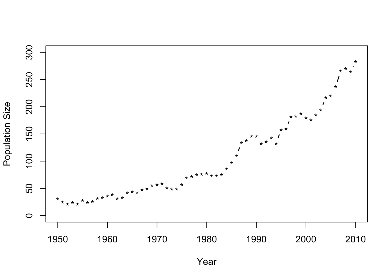 - Ordinary differential equations
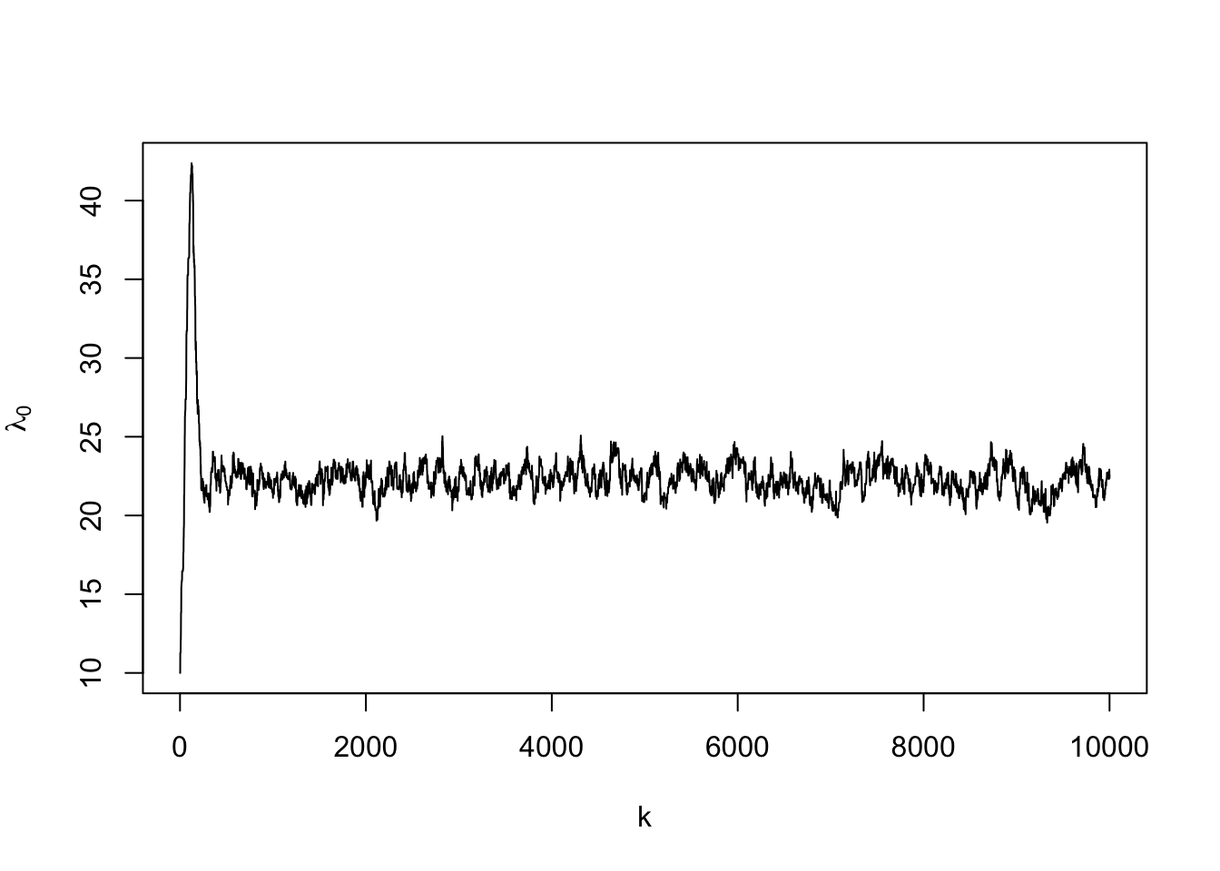
- The expected number of whooping cranes at any given time can be calculated by\[\lambda(t+\Delta t)=\lambda(t)+b(t)-d(t)\:.\]At time t, let the births equal \(b(t)=\beta\Delta t\lambda(t)\) and deaths equal \(d(t)=\alpha\Delta t\lambda(t)\). Then write the equation above as \[\lambda(t+\Delta t)=\lambda(t)+\beta\Delta t\lambda(t)-\alpha\Delta t\lambda(t)\:.\] Now define the growth rate as \(\gamma=\beta-\alpha\) and rewrite as \[\lambda(t+\Delta t)=\lambda(t)+\gamma\Delta t\lambda(t)\:.\] Next write the equation as\[\frac{\lambda(t+\Delta t)-\lambda(t)}{\Delta t}=\gamma\lambda(t)\] and let \[\Delta t\rightarrow0\lim_{\Delta t\rightarrow0}\frac{\lambda(t+\Delta t)-\lambda(t)}{\Delta t}=\gamma\lambda(t)\:.\] Finally replace \(\lim_{\Delta t\rightarrow0}\frac{\lambda(t+\Delta t)-\lambda(t)}{\Delta t}\) with the differential operator\[\frac{d\lambda(t)}{dt}=\gamma\lambda(t)\:.\]
- Solving requires an ODE and initial conditions
- The expected number of whooping cranes in 1949?
- Analytical solution to ODEs \[\lambda(t)=\lambda_{0}e^{\gamma t}\]
- Numerical solution to ODEs
- Finite difference method (replace \(\frac{d\lambda(t)}{dt}\) with \(\frac{\lambda_{t+\Delta t}-\lambda_{t}}{\Delta t}\))
\[\frac{d\lambda(t)}{dt}=\gamma\lambda\]
\[\frac{\lambda_{t+\Delta t}-\lambda_{t}}{\Delta t}=\gamma\lambda\]
\[\lambda_{t+\Delta t}=\lambda_{t}+\gamma\Delta t\lambda_{t}\]
- Ordinary differential equations
- The expected number of whooping cranes at any given time can be calculated by\[\lambda(t+\Delta t)=\lambda(t)+b(t)-d(t)\:.\]At time t, let the births equal \(b(t)=\beta\Delta t\lambda(t)\) and deaths equal \(d(t)=\alpha\Delta t\lambda(t)\). Then write the equation above as \[\lambda(t+\Delta t)=\lambda(t)+\beta\Delta t\lambda(t)-\alpha\Delta t\lambda(t)\:.\] Now define the growth rate as \(\gamma=\beta-\alpha\) and rewrite as \[\lambda(t+\Delta t)=\lambda(t)+\gamma\Delta t\lambda(t)\:.\] Next write the equation as\[\frac{\lambda(t+\Delta t)-\lambda(t)}{\Delta t}=\gamma\lambda(t)\] and let \[\Delta t\rightarrow0\lim_{\Delta t\rightarrow0}\frac{\lambda(t+\Delta t)-\lambda(t)}{\Delta t}=\gamma\lambda(t)\:.\] Finally replace \(\lim_{\Delta t\rightarrow0}\frac{\lambda(t+\Delta t)-\lambda(t)}{\Delta t}\) with the differential operator\[\frac{d\lambda(t)}{dt}=\gamma\lambda(t)\:.\]
- Solving requires an ODE and initial conditions
- The expected number of whooping cranes in 1949?
- Analytical solution to ODEs \[\lambda(t)=\lambda_{0}e^{\gamma t}\]
- Numerical solution to ODEs
- Finite difference method (replace \(\frac{d\lambda(t)}{dt}\) with \(\frac{\lambda_{t+\Delta t}-\lambda_{t}}{\Delta t}\))
\[\frac{d\lambda(t)}{dt}=\gamma\lambda\]
\[\frac{\lambda_{t+\Delta t}-\lambda_{t}}{\Delta t}=\gamma\lambda\]
\[\lambda_{t+\Delta t}=\lambda_{t}+\gamma\Delta t\lambda_{t}\]
- Write out Bayesian statistical model for whooping cranes
y <- df1$N
m.draws <- 10000  #Number of MCMC samples to draw
samples <- as.data.frame(matrix(,m.draws+1,2))
colnames(samples) <- c("gamma","lambda0")
samples[1,] <- c(0,10)  #Starting values for gamma & lambda0

#Monitor acceptance rate for Metropolis-Hastings algorithm
accept <- as.data.frame(matrix(0,m.draws+1,2))
colnames(accept) <- c("gamma","lambda0")

a <- -10 # uniform prior for gamma
b <- 2

c <- 0 # uniform prior for lambda0
d <- 100

gamma.tune <- 0.0007
lambda0.tune <- 0.7


calc.lambda <- function(lambda0,gamma,t.max,dt,t.keep){
  lambda <- matrix(,t.max/dt+1,1)
  lambda[1,] <- lambda0
  for(i in 1:(t.max/dt)){
    lambda[i+1,] <- lambda[i,]*(1+dt*gamma)
  }
  (lambda[-1,])[t.keep]
}

t.max <- length(y)
dt <- 1/12
t.keep <- seq(1,t.max/dt,by=1/dt)


set.seed(4403)
ptm <- proc.time()
for(k in 1:m.draws){

    gamma <- samples[k,1]
    lambda0 <- samples[k,2]
    lambda <- calc.lambda(lambda0,gamma,t.max,dt,t.keep)

    #Sample gamma
    gamma.star <- rnorm(1,gamma,gamma.tune)
    if(gamma.star > a & gamma.star < b){
    lambda.star <- calc.lambda(lambda0,gamma.star,t.max,dt,t.keep)
    mh1 <- sum(dpois(y,lambda.star,log=TRUE)) + dunif(gamma.star,a,b,log=TRUE)
    mh2 <- sum(dpois(y,lambda,log=TRUE)) + dunif(gamma,a,b,log=TRUE)
    R <- min(1,exp(mh1 - mh2))
    if (R > runif(1)){gamma <- gamma.star;lambda <- lambda.star; accept[k+1,1] <- 1}}

    #Sample lambda0
    lambda0.star <- rnorm(1,lambda0,lambda0.tune)
    if(lambda0.star > c & lambda0.star < d){
    lambda.star <- calc.lambda(lambda0.star,gamma,t.max,dt,t.keep)
    mh1 <- sum(dpois(y,lambda.star,log=TRUE)) + dunif(lambda0.star,c,d,log=TRUE)
    mh2 <- sum(dpois(y,lambda,log=TRUE)) + dunif(lambda0,c,d,log=TRUE)
    R <- min(1,exp(mh1 - mh2))
    if (R > runif(1)){lambda0 <- lambda0.star; accept[k+1,2] <- 1}}

    samples[k+1,1] <- gamma
    samples[k+1,2] <- lambda0
    if(k%%1000==0){print(k)}
}
## [1] 1000
## [1] 2000
## [1] 3000
## [1] 4000
## [1] 5000
## [1] 6000
## [1] 7000
## [1] 8000
## [1] 9000
## [1] 10000## user system elapsed
## 10.323 0.185 11.064## gamma lambda0
## 0.4272 0.4332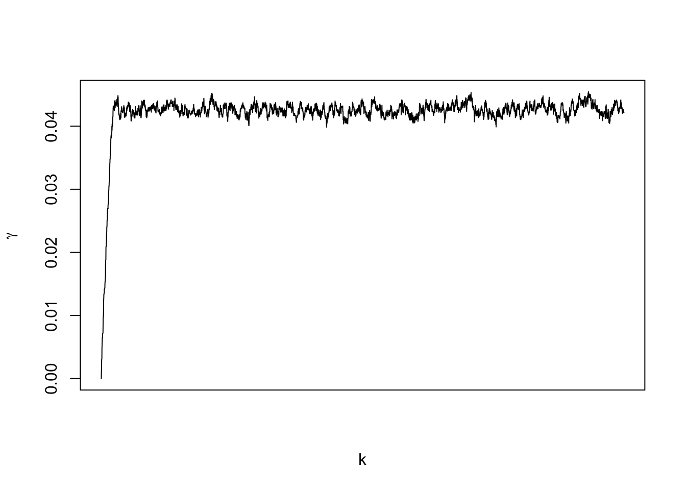
##       gamma     lambda0
## 0.04261365 22.25786503## gamma lambda0
## 2.5% 0.04100095 20.56473
## 97.5% 0.04430795 23.89963t.max <- length(y) + 20
dt <- 1/12
t.keep <- which(seq(1950,2030,by=dt)>=2010)
samples.pred <- matrix(,m.draws+1,length(t.keep))
for(k in 1:(m.draws+1)){
gamma <- samples[k,1]
lambda0 <- samples[k,2]
lambda <- calc.lambda(lambda0,gamma,t.max,dt,t.keep)
y.new <- rpois(length(t.keep),lambda)
samples.pred[k,] <- y.new
}
par(mfrow=c(1,1))
plot(seq(2010,2030,by=dt),colMeans(samples.pred[-c(1:burn.in),]),typ="l",xlab = "Year", ylab = "Population Size",xlim=c(1950,2030),ylim=c(0,700))
lwr.CI <- apply(samples.pred[-c(1:burn.in),],2,FUN=quantile,prob=c(0.025))
upper.CI <- apply(samples.pred[-c(1:burn.in),],2,FUN=quantile,prob=c(0.975))
polygon(c(seq(2010,2030,by=dt),rev(seq(2010,2030,by=dt))),c(lwr.CI,rev(upper.CI)),col=rgb(0.5,0.5,0.5,0.3),border=NA)
points(df1$Winter, df1$N, typ = "p", lwd = 1.5, pch = "*")
legend(x = 1960, y = 600, cex = 1.3, legend = c(expression("E("*y[new]*"|"*y[obs]*")"),"95% CI"), bty = "n",
lty = 1, lwd = 2, col = c("black",rgb(0.5,0.5,0.5,0.5)))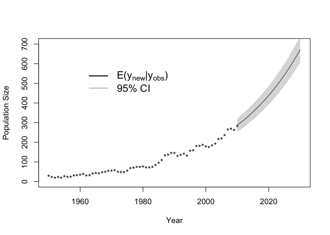
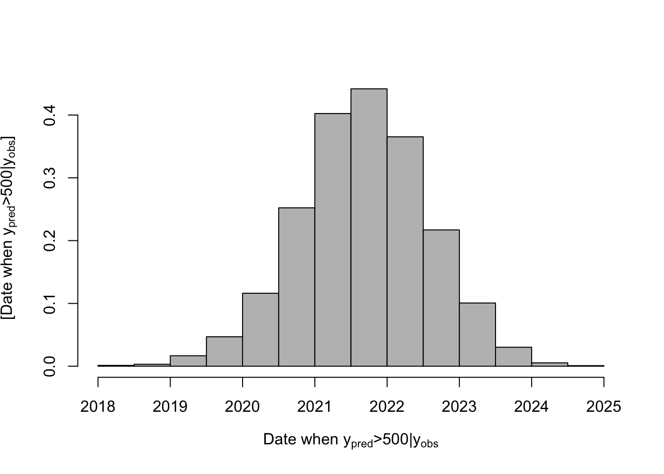
# Posterior distribution of when population size is >500
date.deriv <- seq(2010,2030,by=dt)[apply(samples.pred[-c(1:burn.in),],1,FUN=function(x){which(x>=500)[1]})]
hist(date.deriv,col="grey",freq=FALSE,main="",xlab=expression("Date when "* y[pred] *">500|"*y[obs]),
     ylab=expression("[Date when "* y[pred] *">500|"*y[obs]*"]"))