24 Activity 4 (Guide)

For this assignment let $[a]$ be a beta distribution with $\alpha=2$ and $\beta=1$ (i.e., $a\sim\text{beta}(\alpha=2,\beta=1)$).

A common choice for the proposal distribution in the Metropolis algorithm is the random walk proposal. In this approach, the proposed state $\theta^{\star}$ is generated by adding a random perturbation to the current state $\theta$, such that

$$\theta^{\star} = \theta^{(k-1)} + \epsilon,$$

where $\epsilon$ is drawn from a symmetric distribution, often a normal distribution $\mathcal{N}(0, \sigma^2)$. This means, at every iteration, you will take a random draw from a proposal distribution, $\theta^{\star} \sim \mathcal{N}(\theta^{(k-1)}, \sigma^2_{tune})$. Since the proposal distribution is symmetric, meaning $q(\theta^{\star} \mid \theta^{(k-1)}) = q(\theta^{(k-1)} \mid \theta^{\star})$, the acceptance probability simplifies to

$$p = \min\left(1, \frac{\pi(\theta^{\star})}{\pi(\theta^{(k-1)})} \right).$$

The step size $\sigma^_{tune}$ plays a crucial role in the efficiency of the algorithm. If $\sigma^_{tune}$ is too small, the chain explores the space slowly, leading to high autocorrelation. If $\sigma^_{tune}$ is too large, proposals are frequently rejected, reducing efficiency. Tuning $\sigma^_{tune}$ appropriately ensures effective mixing of the Markov chain.

To begin I’ve made a function to perform the Metropolis-Hasting algorithm, which I can reuse for each of the following questions.

metropolis_hastings <- function(n_samples, sigma2_tune) {
  x <- numeric(n_samples)
  x[1] <- runif(1)  # Initialize
  
  for (i in 2:n_samples) {
    # A "random walk" or Metropolis proposal is a Normal distribution with
    # the mean at the previous value and the var/sd deciding how big of a 
    # "step" away from the mean you take
    proposal <- rnorm(1, mean = x[i - 1], sd = sqrt(sigma2_tune))
    
    # Compute Metropolis-Hastings ratio
    acceptance_ratio <- dbeta(proposal, 2, 1) / dbeta(x[i - 1], 2, 1)
    acceptance_ratio <- min(1, acceptance_ratio)  # Ensure it's in [0,1]
    
    if (runif(1) < acceptance_ratio) {
      x[i] <- proposal
    } else {
      x[i] <- x[i - 1]
    }
  }
  return(x)
}

Now that the preliminary steps are taken care of, we can move forward answering the questions.

1. Using a Metropolis-Hastings to draw 5000 samples from $[a]$ using a Metropolis proposal with $\sigma^2_{tune}=0.0001$. Also, write out the M-H ratio and simplify.

Before we begin, it is important to note that we are sampling from $[a]$ and NOT the posterior of a Bayesian model. Thus Metropolis-Hastings ratio, from page 34 of Bringing Bayesian Methods To Life, is

$$mh = \frac{[\theta^{\star}][\theta^{(k-1)} \mid \theta^{\star}]}{[\theta^{(k-1)}][\theta^{\star} \mid \theta^{(k-1)}]}$$ Note that, because the proposal distribution is symmetric, then $[\theta^{\star} \mid \theta^{(k-1)}] = [\theta^{(k-1)} \mid \theta^{\star}]$. Because of this, our mh-ratio simplifies to

$$mh = \frac{[\theta^{\star}]}{[\theta^{(k-1)}]}$$

If we plug in the target density function (i.e., the pdf of a beta(2,1)), we can further reduce this to $$\begin{aligned} mh &= \frac{2 \theta^{\star}}{2 \theta^{(k-1)}} \\ &= \frac{\theta^{\star}}{\theta^{(k-1)}} \end{aligned}$$

The R code for question #1 is below.

set.seed(1234) # so you can get the same results, if you're following at home

n_samples <- 5000

small_step <- metropolis_hastings(n_samples, sigma2_tune = 0.0001)

2. Discard the first 1000 samples drawn in question 1, then calculate the mean. Write out the integral you’re approximating.

Let’s begin with the integral we are approximating. The integral is written below, along with its analytical solution. $$\begin{aligned} \mathbb{E} &= \int_0^1 a [a] da \\ &= \int_0^1 2a^2 da \\ &= \frac{2}{3} \end{aligned}$$

burn_in <- 1000

mean_small <- mean(small_step[-(1:burn_in)])
mean_small

## [1] 0.3436342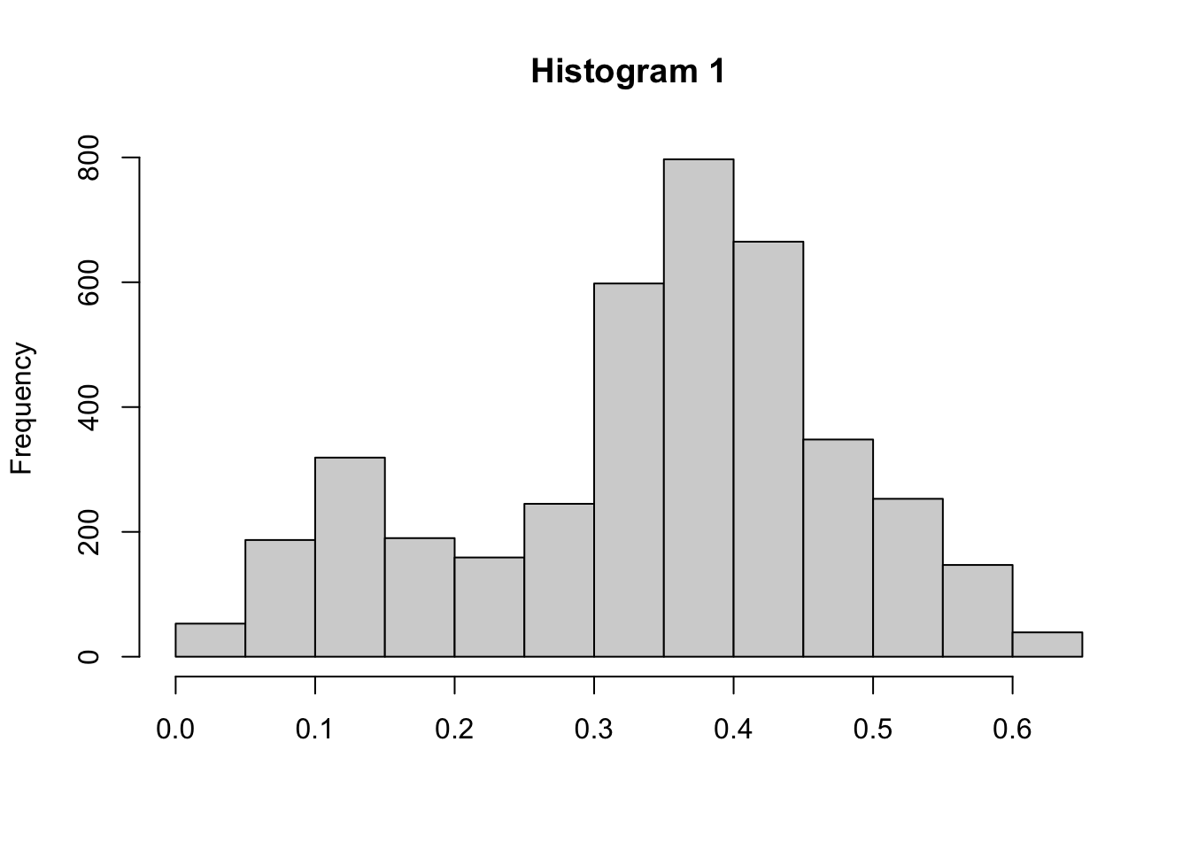

hist(small_step[-(1:burn_in)],
     main = "Histogram 1", xlab ="",breaks = 15)

3. Repeat question 1 with $\sigma^2_{tune}=0.25$.

mid_step <- metropolis_hastings(n_samples, sigma2_tune = 0.25)

4. Find the mean of the samples in question 3, removing the first 1000 samples for burn-in.

mean_mid <- mean(mid_step[-(1:burn_in)])
mean_mid

## [1] 0.6745351

hist(mid_step[-(1:burn_in)],
     main = "Histogram 2", xlab ="", breaks = 15)

5. Repeat question qith $\sigma^2_{tune} =10$

big_step <- metropolis_hastings(n_samples, sigma2_tune = 10)

6. Find the mean of the samples in question 5, removing the first 1000 samples for burn-in.

mean_big <- mean(big_step[-(1:burn_in)])
mean_big

## [1] 0.6842496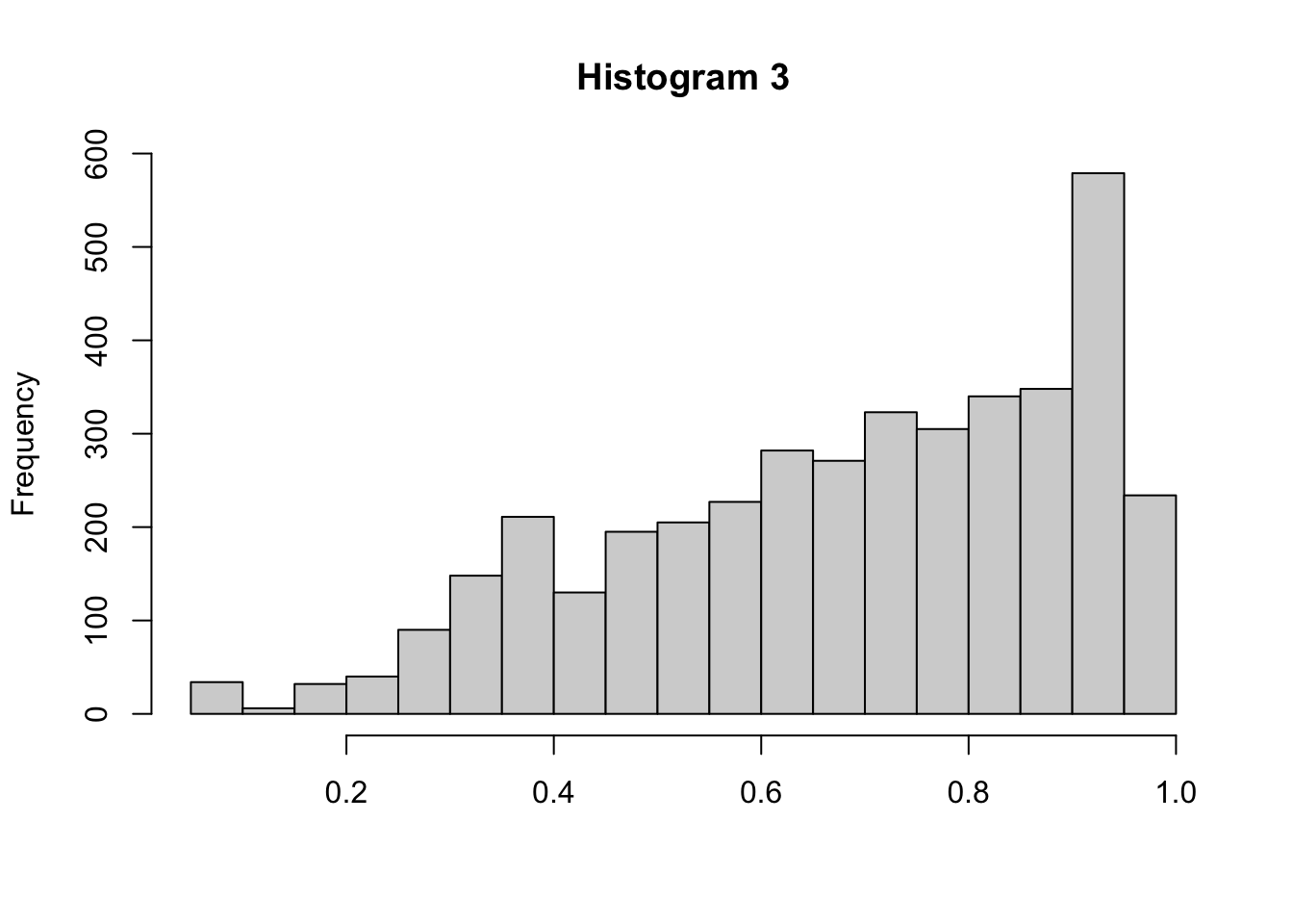

hist(big_step[-(1:burn_in)], 
     main = "Histogram 3", xlab ="", breaks = 15)

7. Compare the numerical values of the MC approximation to the integrals in questions 2, 4, and 6.

This activity always makes me think of Goldilocks and the Three Bears. What we are trying to do is find that “Baby Bear” value for $\sigma^2_{tune}$ so that the proposal will walk across all values of $a$. If $\sigma^2_{tune}$ is too small (question 1 and 2), then it will take too long and move too slow (see Histogram 1). Alternatively, when $\sigma^2_{tune}$ is too large (question 5 and 6), then the proposal distribution will take too big of “steps” and end up jumping to values that are not realistic (see Histogram 3). Only when $\sigma^2_{tune}$ is tuned just right will we get samples that truly reflect the density of $a$ (see Histogram 2).