15 Day 15 (March 11)

15.1 Announcements

• Questions about activity 5?

• Guide to activity 4 is coming

• Read Chs. 11 and 12

• Start reading Ch 16 (time series)

• Selected questions/clarifications from journals

  • All questions/comments below are about retirement example
  • Why would you want to use a model based on assumptions rather than data?
  • Prior predictions seems useful only if there is some pre-existing data/information.
  • How did I get the prior for r in the retirement example?
  • But you used data to in the retirement example…
  • Translating this to another example, what if I didn’t know the “starting value”

15.2 Bayesian prediction

• Prior prediction vs. posterior prediction
  • Prior prediction is used before fitting your model to data. It is used as a model checking tool (e.g., to see if priors are reasonable) or to do prediction if you have little or no data.
  • Posterior prediction is more typically what you think of as prediction. It is done after fitting your model to data.
• Example revisiting white lupine data set from day 1
  • Details of data and analysis from Palmero et al. (2024)
  • Live example

15.3 Time series

What is a time series? - One damned thing after another (maybe Fisher) - Spatio-temporal data collected at a single point in space over multiple time points - Spatio-temporal data aggregated over space - Any data set/model that has dependence in residual errors over time

• Phenomenological vs. mechanistic mathematical models
  • Recall my retirement example?
  • Population growth example of whooping cranes

url<-"https://www.dropbox.com/s/sr2411umm053vcq/Butler%20et%20al.%20Table%201.csv?dl=1"
df1 <- read.csv(url)
plot(df1$Winter, df1$N, xlab = "Year", ylab = "Population Size",
ylim = c(0, 300), typ = "b", lwd = 1.5, pch = "*")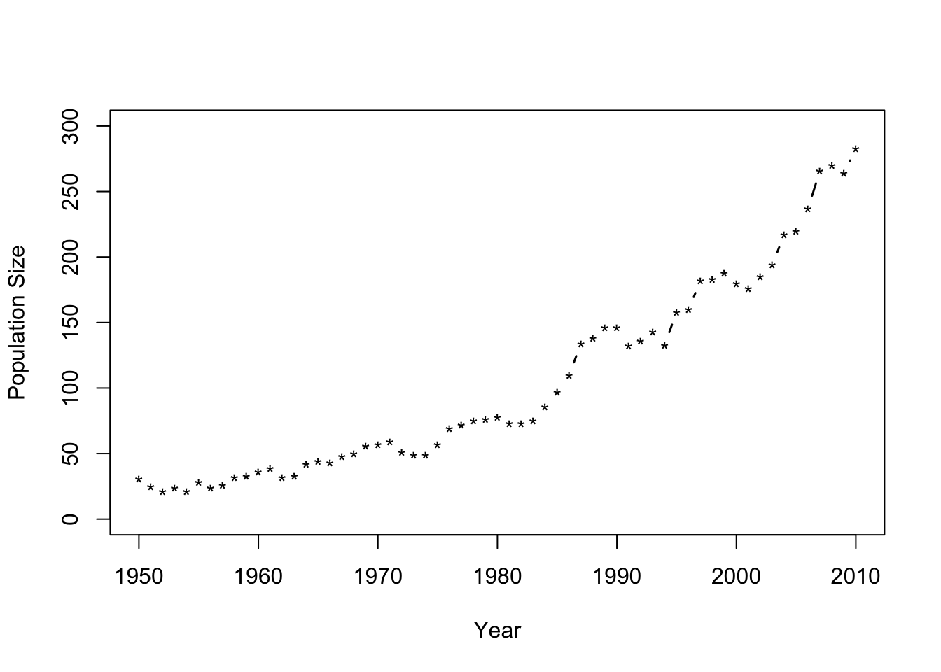

• Example: population growth in continuous time
  • Ordinary differential equations
  • The expected number of whooping cranes at any given time can be calculated by $$\lambda(t+\Delta t)=\lambda(t)+b(t)-d(t)\:.$$ At time t, let the births equal $b(t)=\beta\Delta t\lambda(t)$ and deaths equal $d(t)=\alpha\Delta t\lambda(t)$. Then write the equation above as $$\lambda(t+\Delta t)=\lambda(t)+\beta\Delta t\lambda(t)-\alpha\Delta t\lambda(t)\:.$$ Now define the growth rate as $\gamma=\beta-\alpha$ and rewrite as $$\lambda(t+\Delta t)=\lambda(t)+\gamma\Delta t\lambda(t)\:.$$ Next write the equation as $$\frac{\lambda(t+\Delta t)-\lambda(t)}{\Delta t}=\gamma\lambda(t)$$ and let $$\Delta t\rightarrow0\lim_{\Delta t\rightarrow0}\frac{\lambda(t+\Delta t)-\lambda(t)}{\Delta t}=\gamma\lambda(t)\:.$$ Finally replace $\lim_{\Delta t\rightarrow0}\frac{\lambda(t+\Delta t)-\lambda(t)}{\Delta t}$ with the differential operator $$\frac{d\lambda(t)}{dt}=\gamma\lambda(t)\:.$$
  • Solving requires an ODE and initial conditions
    • The expected number of whooping cranes in 1949?
  • Analytical solution to ODEs $$\lambda(t)=\lambda_{0}e^{\gamma t}$$
  • Numerical solution to ODEs
    • Finite difference method (replace $\frac{d\lambda(t)}{dt}$ with $\frac{\lambda_{t+\Delta t}-\lambda_{t}}{\Delta t}$) $$\frac{d\lambda(t)}{dt}=\gamma\lambda$$ $$\frac{\lambda_{t+\Delta t}-\lambda_{t}}{\Delta t}=\gamma\lambda$$ $$\lambda_{t+\Delta t}=\lambda_{t}+\gamma\Delta t\lambda_{t}$$
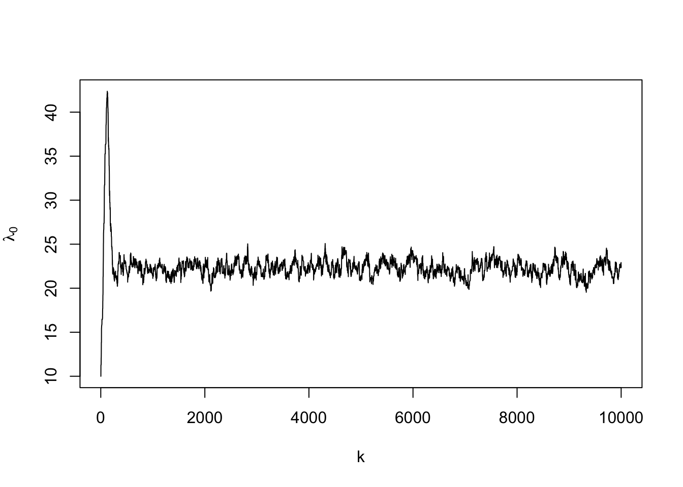
  • Write out Bayesian statistical model for whooping cranes

y <- df1$N
m.draws <- 10000  #Number of MCMC samples to draw
samples <- as.data.frame(matrix(,m.draws+1,2))
colnames(samples) <- c("gamma","lambda0")
samples[1,] <- c(0,10)  #Starting values for gamma & lambda0

#Monitor acceptance rate for Metropolis-Hastings algorithm
accept <- as.data.frame(matrix(0,m.draws+1,2)) 
colnames(accept) <- c("gamma","lambda0")

a <- -10 # uniform prior for gamma
b <- 2

c <- 0 # uniform prior for lambda0
d <- 100

gamma.tune <- 0.0007
lambda0.tune <- 0.7


calc.lambda <- function(lambda0,gamma,t.max,dt,t.keep){
  lambda <- matrix(,t.max/dt+1,1)
  lambda[1,] <- lambda0
  for(i in 1:(t.max/dt)){
    lambda[i+1,] <- lambda[i,]*(1+dt*gamma)
  }
  (lambda[-1,])[t.keep]
}

t.max <- length(y)
dt <- 1/12
t.keep <- seq(1,t.max/dt,by=1/dt)
    

set.seed(4403)
ptm <- proc.time()
for(k in 1:m.draws){
    
    gamma <- samples[k,1]
    lambda0 <- samples[k,2]
    lambda <- calc.lambda(lambda0,gamma,t.max,dt,t.keep)
  
    #Sample gamma
    gamma.star <- rnorm(1,gamma,gamma.tune)
    if(gamma.star > a & gamma.star < b){
    lambda.star <- calc.lambda(lambda0,gamma.star,t.max,dt,t.keep)
    mh1 <- sum(dpois(y,lambda.star,log=TRUE)) + dunif(gamma.star,a,b,log=TRUE)
    mh2 <- sum(dpois(y,lambda,log=TRUE)) + dunif(gamma,a,b,log=TRUE)
    R <- min(1,exp(mh1 - mh2))
    if (R > runif(1)){gamma <- gamma.star;lambda <- lambda.star; accept[k+1,1] <- 1}}
    
    #Sample lambda0
    lambda0.star <- rnorm(1,lambda0,lambda0.tune)
    if(lambda0.star > c & lambda0.star < d){
    lambda.star <- calc.lambda(lambda0.star,gamma,t.max,dt,t.keep)
    mh1 <- sum(dpois(y,lambda.star,log=TRUE)) + dunif(lambda0.star,c,d,log=TRUE)
    mh2 <- sum(dpois(y,lambda,log=TRUE)) + dunif(lambda0,c,d,log=TRUE)
    R <- min(1,exp(mh1 - mh2))
    if (R > runif(1)){lambda0 <- lambda0.star; accept[k+1,2] <- 1}}
    
    samples[k+1,1] <- gamma
    samples[k+1,2] <- lambda0
    if(k%%1000==0){print(k)}
}

## [1] 1000
## [1] 2000
## [1] 3000
## [1] 4000
## [1] 5000
## [1] 6000
## [1] 7000
## [1] 8000
## [1] 9000
## [1] 10000

proc.time() - ptm 

##    user  system elapsed 
##   8.917   0.152   9.163

colMeans(accept[-1,]) 

##   gamma lambda0 
##  0.4272  0.4332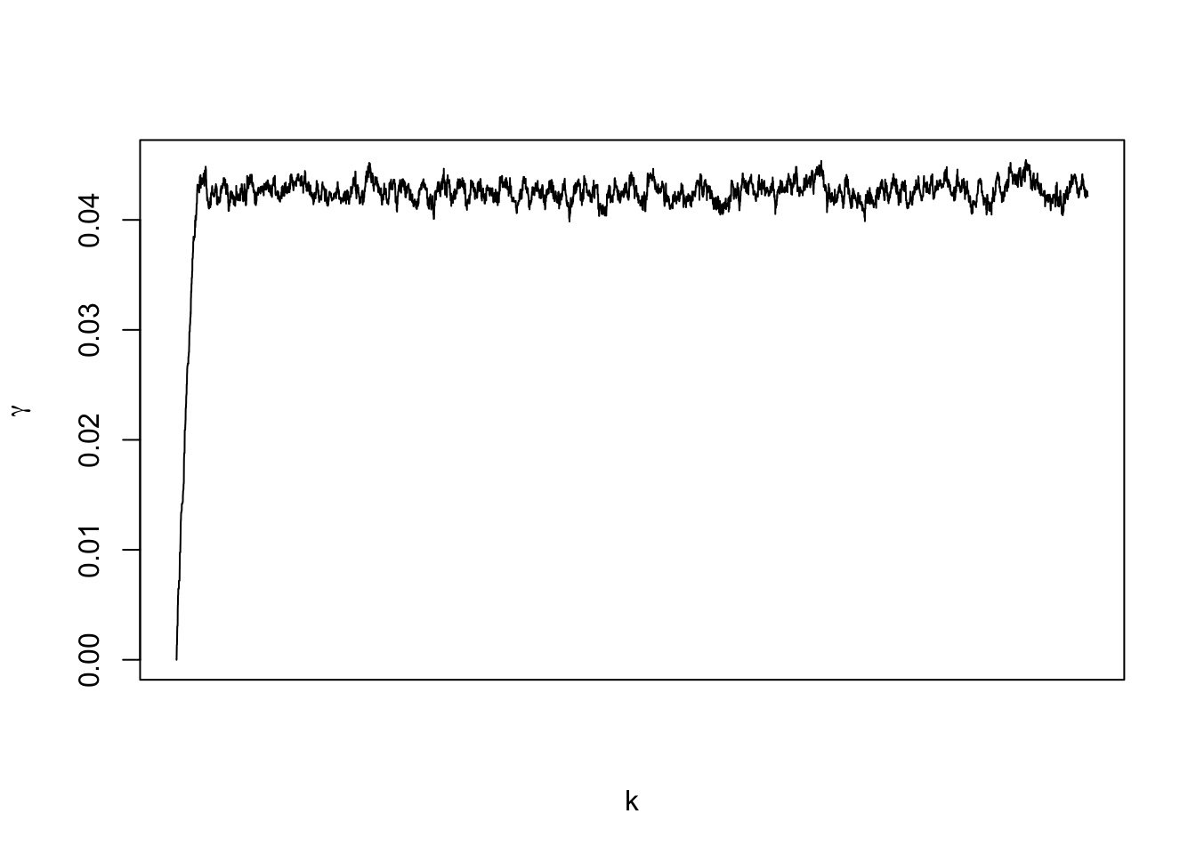

#Make sure to check trace plots
plot(samples[,1],typ="l",xlab="k",ylab=expression(gamma),xaxt='n')

plot(samples[,2],typ="l",xlab="k",ylab=expression(lambda[0]))

burn.in <- 1000
# E() of gamma & lambda0
colMeans(samples[-c(1:burn.in),])  

##       gamma     lambda0 
##  0.04261365 22.25786503

# 95% Equal-tailed CIs
apply(samples[-c(1:burn.in),],2,FUN=quantile,prob=c(0.025,0.975)) 

##            gamma  lambda0
## 2.5%  0.04100095 20.56473
## 97.5% 0.04430795 23.89963

t.max <- length(y) + 20
dt <- 1/12
t.keep <- which(seq(1950,2030,by=dt)>=2010)
 
samples.pred <- matrix(,m.draws+1,length(t.keep))

for(k in 1:(m.draws+1)){
    gamma <- samples[k,1]
    lambda0 <- samples[k,2]
    lambda <- calc.lambda(lambda0,gamma,t.max,dt,t.keep)
    y.new <- rpois(length(t.keep),lambda)
    samples.pred[k,] <- y.new
}

par(mfrow=c(1,1))
plot(seq(2010,2030,by=dt),colMeans(samples.pred[-c(1:burn.in),]),typ="l",xlab = "Year", ylab = "Population Size",xlim=c(1950,2030),ylim=c(0,700))
lwr.CI <- apply(samples.pred[-c(1:burn.in),],2,FUN=quantile,prob=c(0.025))
upper.CI <- apply(samples.pred[-c(1:burn.in),],2,FUN=quantile,prob=c(0.975))
polygon(c(seq(2010,2030,by=dt),rev(seq(2010,2030,by=dt))),c(lwr.CI,rev(upper.CI)),col=rgb(0.5,0.5,0.5,0.3),border=NA)
points(df1$Winter, df1$N, typ = "p", lwd = 1.5, pch = "*")
legend(x = 1960, y = 600, cex = 1.3, legend = c(expression("E("*y[new]*"|"*y[obs]*")"),"95% CI"), bty = "n",
lty = 1, lwd = 2, col = c("black",rgb(0.5,0.5,0.5,0.5)))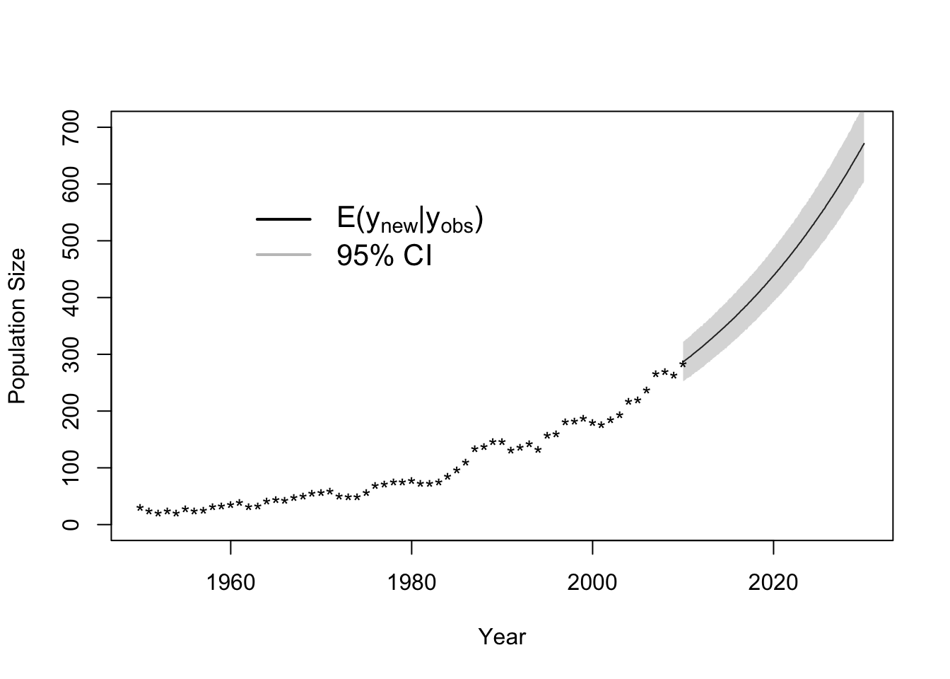

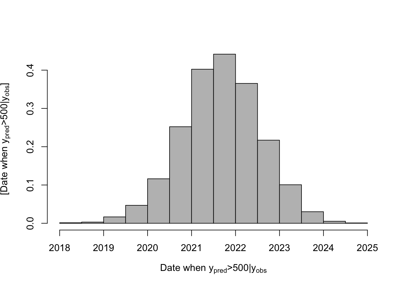
# Posterior distribution of when population size is >500
date.deriv <- seq(2010,2030,by=dt)[apply(samples.pred[-c(1:burn.in),],1,FUN=function(x){which(x>=500)[1]})]
hist(date.deriv,col="grey",freq=FALSE,main="",xlab=expression("Date when "* y[pred] *">500|"*y[obs]),
     ylab=expression("[Date when "* y[pred] *">500|"*y[obs]*"]"))