1 Day 1 (January 21)

1.1 Welcome and preliminaries

About me
Teaching Assistant
Course website
- How I will use Canvas
  - Grades, journal and project submissions only
Syllabus
- Required and Recomended material
- Statistical programming languages
- Reproducibility requirement (data analysis and computing can be successfully repeated)
- Academic Honesty: working in groups, sharing code, etc.
- Grades
- Topics
Who is in this class?
- Group work and collaboration

url <- "https://www.dropbox.com/scl/fi/yy44rp2bx263d9byltk3m/students_STAT_768.csv?rlkey=zbt60fpkl9ta9d3uqysu3vbtf&dl=1"
df <- read.csv(url)

par(mar=c(13,2,2,2))
plot(rev(sort(table(df$degreeProgram))),las=2,xlab="",ylab="Number of students",ylim=c(0,8))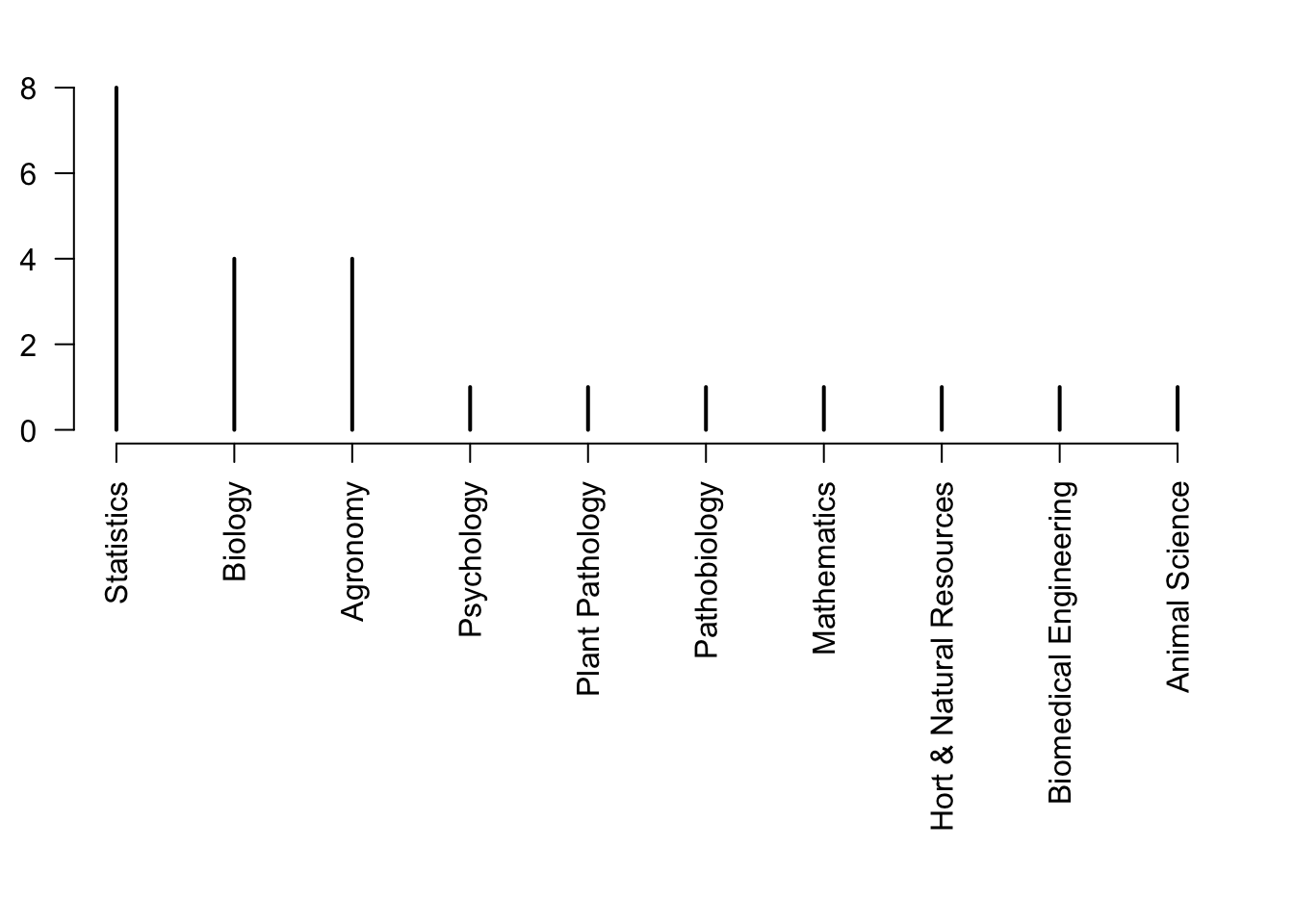

par(mar=c(13,2,2,2))
plot(rev(sort(table(df$classLevel))),las=2,xlab="",ylab="Number of students",ylim=c(0,15))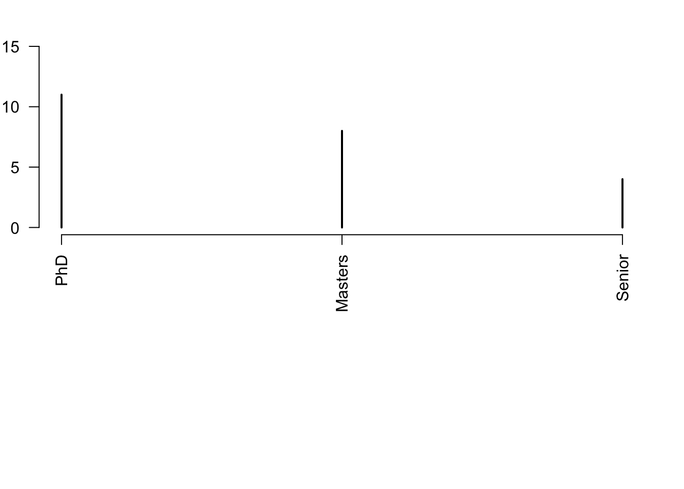

1.2 Intro to Bayesian statistical modelling

What is data?
- Something in the real world that you can, in some way, observe and measure with or without error
What is a statistic?
- A function of the data
What is a model?
- Mathematical models
- Statistical models
What is a parameter?
- Part of a statistical model that is usually unknown and must be assumed or estimated.
What is the goal of Bayesian statistics?
- Obtain the distribution of potentially unrecordable random variables given recorded random variables

1.3 Example with linear models

What is a model?
What is a linear model?
- Most widely used model in science, engineering, and statistics.
- Scalar form: $y_i=\beta_{0}+\beta_{1}x_{i}+\varepsilon_i$
- Which part of the model is the mathematical model.
- Which part of the model makes the linear model a “statistical” model.
- Visual

1.4 Estimation and inference

Three options to estimate $\beta_0$ and $\beta_1$
- Minimize a loss function
- Maximize a likelihood function
- Find the posterior distribution
- Each option requires different assumptions

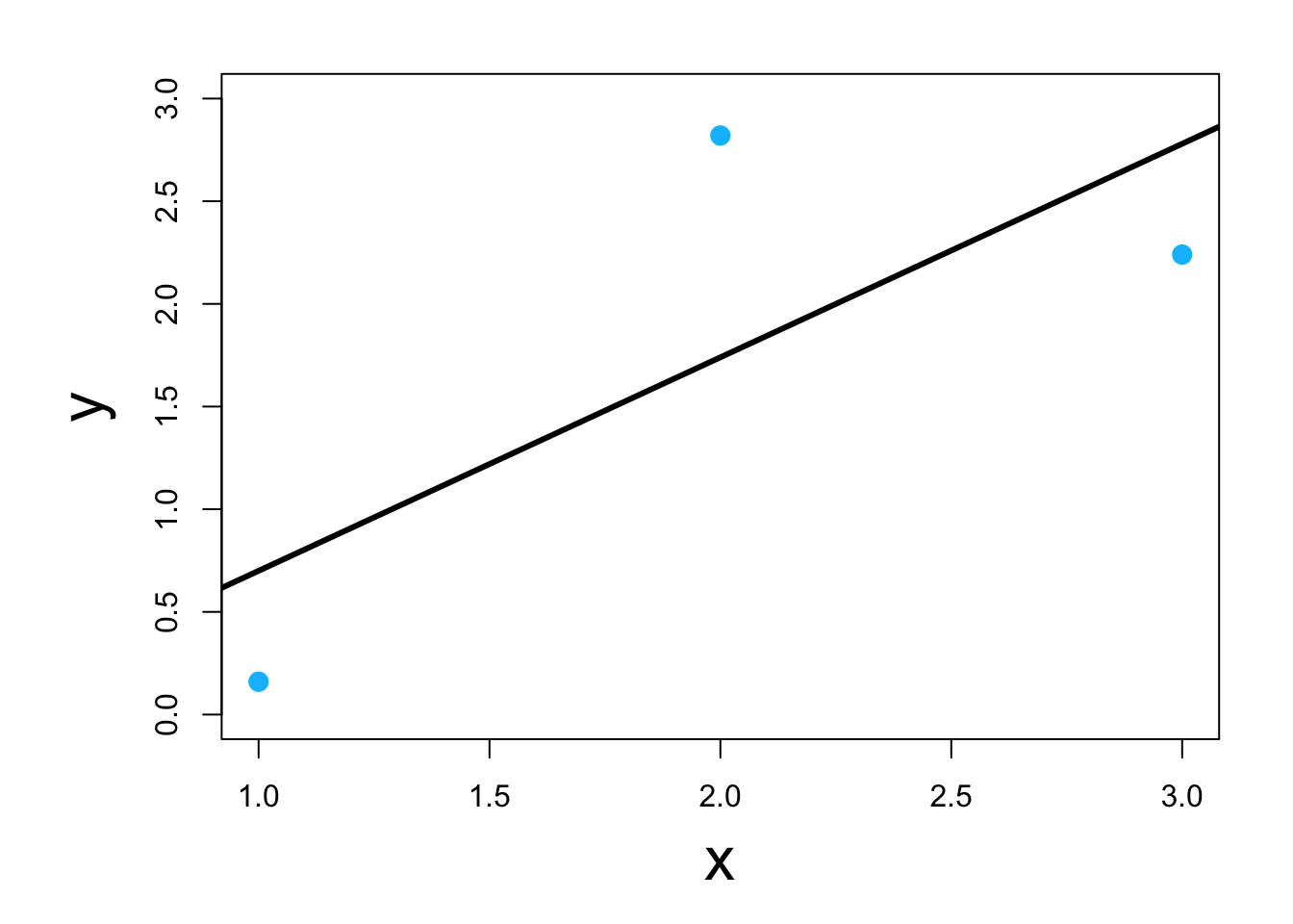
1.5 Loss function approach

Define a measure of discrepancy between the data and the mathematical model
- Find the values of $\beta_0$ and $\beta_1$ that makes $\beta_{0}+\beta_{1}x_i$ “closest” to $y_i$
- Visual

Real data example

Details from Palmero et al. (2024)

# Preliminary steps
url <- "https://www.dropbox.com/scl/fi/2qph4g9vnacibr73edrsb/Fig3_data.csv?rlkey=n48lbrv2zf2z5k1uja1393sof&dl=1"
df.all <- read.csv(url)
df.fp <- df.all[which(df.all$Scenario=="Scenario A"),]

# Plot data for field pea
plot(df.fp$Ndfa,df.fp$PartNbalance,
 xlab="Ndfa (%)",ylab="Partial N balance (kg/ha)",
 xlim=c(0,110),ylim=c(-100,200),main="Field pea")
abline(a=0,b=0,col="gold",lwd=3)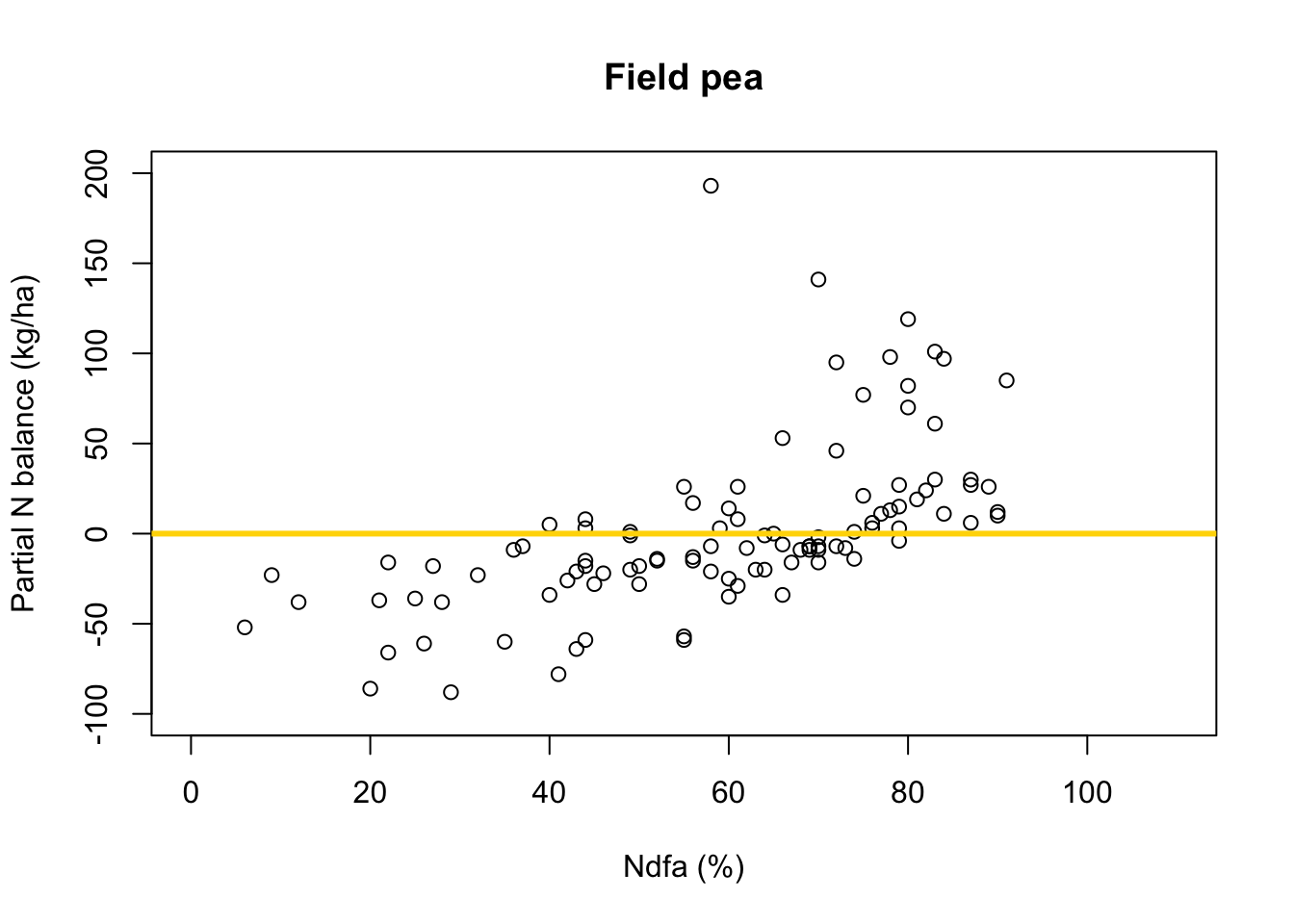

Fit linear model to data using least squares

# Fit simple linear regression model using least squares
m1 <- lm(PartNbalance ~ Ndfa,data=df.fp)

What value of Ndfa is needed to achieve a neutral N balance?

beta0.hat <- as.numeric(coef(m1)[1])
beta1.hat <- as.numeric(coef(m1)[2])
theta.hat <- -beta0.hat/beta1.hat
theta.hat

## [1] 58.26843

Visual representation of $\theta$

# Plot data, line of best fit and theta 
plot(df.fp$Ndfa,df.fp$PartNbalance,
 xlab="Ndfa (%)",ylab="Partial N balance (kg/ha)",
 xlim=c(0,110),ylim=c(-100,200),main="Field pea")
abline(a=0,b=0,col="gold",lwd=3)
abline(m1,col="red",lwd=3)
abline(v=58,lwd=3,lty=2,col="green")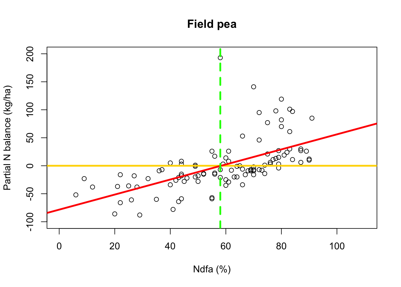

1.6 Likelihood-based approach

Assume that $y_i=\beta_{0}+\beta_{1}x_{i}+\varepsilon_i$ and $\varepsilon_i\sim \text{N}(0,\sigma^2)$
Maximum likelihood estimation for the linear model
- Visual
We added assumptions to our model, so what else do we get?
- Full likelihood-based statistical inference (e.g, p-values, confidence intervals, prediction intervals, etc)

Real data example

Fit linear model to data using using maximum likelihood estimation

library(nlme)
# Fit simple linear regression model using maximum likelihood estimation
m2 <- gls(PartNbalance ~ Ndfa,data=df.fp,method="ML")

What value of Ndfa is needed to achieve a neutral N balance?

# Use maximum likelihood estimate (MLE) to obtain estimate of theta
beta0.hat <- as.numeric(coef(m2)[1])
beta1.hat <- as.numeric(coef(m2)[2])
theta.hat <- -beta0.hat/beta1.hat
theta.hat

## [1] 58.26843

# Use delta method to obtain approximate approximate standard errors and
# then construct Wald-type confidence intervals
library(msm)
theta.se <- deltamethod(~-x1/x2, mean=coef(m2), cov=vcov(m2))

theta.ci <- c(theta.hat-1.96*theta.se,theta.hat+1.96*theta.se)
theta.ci

## [1] 52.88317 63.65370

Visual representation of $\theta$

# Plot data, line of best fit and theta 
plot(df.fp$Ndfa,df.fp$PartNbalance,
 xlab="Ndfa (%)",ylab="Partial N balance (kg/ha)",
 xlim=c(0,110),ylim=c(-100,200),main="Field pea")
abline(a=0,b=0,col="gold",lwd=3)
abline(m1,col="red",lwd=3)
abline(v=58.3,lwd=3,lty=2,col="green") 
abline(v=52.9,lwd=1,lty=2,col="green") 
abline(v=63.7,lwd=1,lty=2,col="green")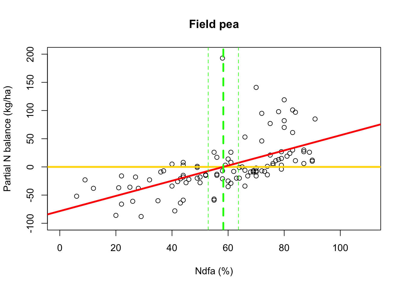

1.7 Bayesian approach

Assume that $y_i=\beta_{0}+\beta_{1}x_{i}+\varepsilon_i$ with $\varepsilon_i\sim \text{N}(0,\sigma^2)$ , $\beta_{0}\sim \text{N}(0,10^6)$ and $\beta_{1}\sim \text{N}(0,10^6)$
Statistical inference
- Using Bayes rule (Bayes 1763) we can obtain the joint posterior distribution $[\beta_0,\beta_1,\sigma_{\varepsilon}^{2}|\mathbf{y}]=\frac{[\mathbf{y}|\beta_0,\beta_1,\sigma_{\varepsilon}^{2}][\beta_0][\beta_1][\sigma_{\varepsilon}^{2}]}{\int\int\int [\mathbf{y}|\beta_0,\beta_1,\sigma_{\varepsilon}^{2}][\beta_0][\beta_1][\sigma_{\varepsilon}^{2}]d\beta_0d\beta_1,d\sigma_{\varepsilon}^{2}}$
  - Statistical inference about a paramters is obtained from the marginal posterior distributions $[\beta_0|\mathbf{y}]=\int[\beta_0,\beta_1,\sigma_{\varepsilon}^{2}|\mathbf{y}]d\beta_1d\sigma_{\varepsilon}^{2}$ $[\beta_1|\mathbf{y}]=\int[\beta_0,\beta_1,\sigma_{\varepsilon}^{2}|\mathbf{y}]d\beta_0d\sigma_{\varepsilon}^{2}$ $[\sigma_{\varepsilon}^{2}|\mathbf{y}]=\int[\beta_0,\beta_1,\sigma_{\varepsilon}^{2}|\mathbf{y}]d\beta_0d\beta_1$
  - Derived quantities can be obtained by transformations of the joint posterior

Computations

Using a Markov chain Monte Carlo algorithm (see Ch.11 in Hooten and Hefley 2019)

norm.reg.mcmc <- function(y,X,beta.mn,beta.var,s2.mn,s2.sd,n.mcmc){

  #
  #  Code Box 11.1
  #

  ###
  ### Subroutines 
  ###

  library(mvtnorm)

  invgammastrt <- function(igmn,igvar){
q <- 2+(igmn^2)/igvar
r <- 1/(igmn*(q-1))
list(r=r,q=q)
  }

  invgammamnvr <- function(r,q){  #  This fcn is not necessary
mn <- 1/(r*(q-1))
vr <- 1/((r^2)*((q-1)^2)*(q-2))
list(mn=mn,vr=vr)
  }

  ###
  ### Hyperpriors
  ###

  n=dim(X)[1]
  p=dim(X)[2]
  r=invgammastrt(s2.mn,s2.sd^2)$r
  q=invgammastrt(s2.mn,s2.sd^2)$q
  Sig.beta.inv=diag(p)/beta.var

  beta.save=matrix(0,p,n.mcmc)
  s2.save=rep(0,n.mcmc)
  Dbar.save=rep(0,n.mcmc)
  y.pred.mn=rep(0,n)

  ###
  ### Starting Values
  ###

  beta=solve(t(X)%*%X)%*%t(X)%*%y

  ###
  ### MCMC Loop
  ###

  for(k in 1:n.mcmc){


###
### Sample s2
###

tmp.r=(1/r+.5*t(y-X%*%beta)%*%(y-X%*%beta))^(-1)
tmp.q=n/2+q

s2=1/rgamma(1,tmp.q,,tmp.r) 

###
### Sample beta
###

tmp.var=solve(t(X)%*%X/s2 + Sig.beta.inv)
tmp.mn=tmp.var%*%(t(X)%*%y/s2 + Sig.beta.inv%*%beta.mn)

beta=as.vector(rmvnorm(1,tmp.mn,tmp.var,method="chol"))

###
### Save Samples
###

beta.save[,k]=beta
s2.save[k]=s2

  }

  ###
  ###  Write Output
  ###

  list(beta.save=beta.save,s2.save=s2.save,y=y,X=X,n.mcmc=n.mcmc,n=n,r=r,q=q,p=p)

}

Model fitting

MCMC

samples <- norm.reg.mcmc(y = df.fp$PartNbalance,X = model.matrix(~ Ndfa,data=df.fp),
                      beta.mn = c(0,0),beta.var=c(10^6,10^6),
                      s2.mn = 10, s2.sd = 10^6,
                      n.mcmc = 5000)

burn.in <- 1000
# Look a histograms of posterior distributions
par(mfrow=c(2,1),mar=c(5,6,1,1))
hist(samples$beta.save[1,-c(1:1000)],xlab=expression(beta[0]*"|"*bold(y)),ylab=expression("["*beta[0]*"|"*bold(y)*"]"),freq=FALSE,col="grey",main="",breaks=30)
hist(samples$beta.save[2,-c(1:1000)],xlab=expression(beta[1]*"|"*bold(y)),ylab=expression("["*beta[1]*"|"*bold(y)*"]"),freq=FALSE,col="grey",main="",breaks=30)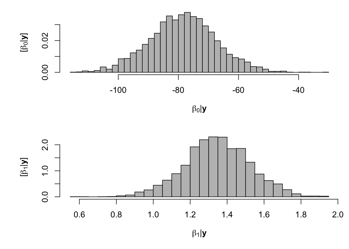

What value of Ndfa is needed to achieve a neutral N balance?

hist(-samples$beta.save[1,-c(1:1000)]/samples$beta.save[2,-c(1:1000)],xlab=expression(theta*"|"*bold(y)),ylab=expression("["*theta*"|"*bold(y)*"]"),freq=FALSE,col="grey",main="",breaks=30)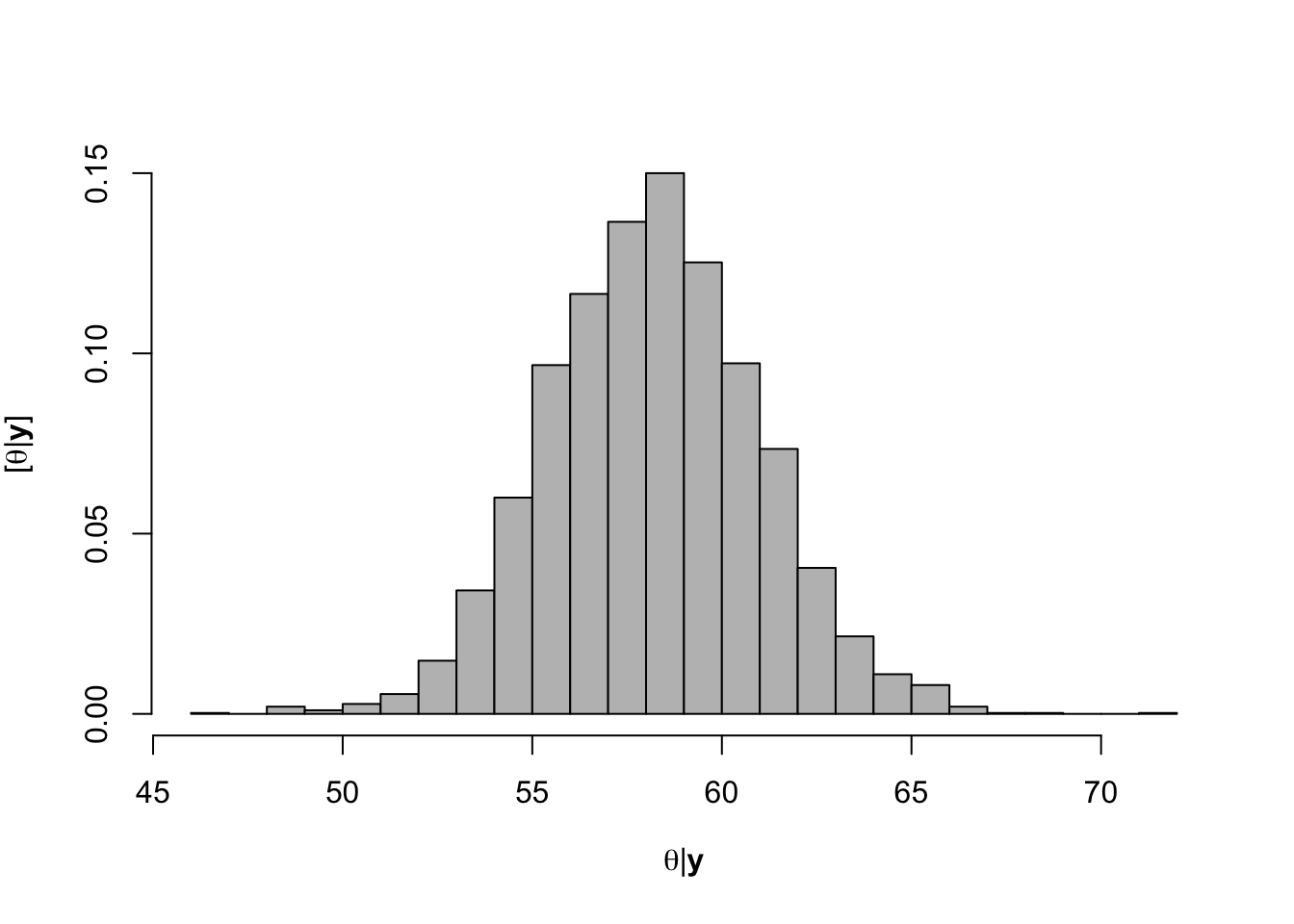

# Expected value (mean) of theta        
mean(-samples$beta.save[1,]/samples$beta.save[2,])

## [1] 58.28103

# 95% credible intervals for theta
quantile(-samples$beta.save[1,]/samples$beta.save[2,],prob=c(0.025,0.975))

##     2.5%    97.5% 
## 52.60634 63.72670

Visual representation of posterior distribuiton of theta $\theta$

# Plot data and theta 
plot(df.fp$Ndfa,df.fp$PartNbalance,
 xlab="Ndfa (%)",ylab="Partial N balance (kg/ha)",
 xlim=c(0,110),ylim=c(-100,200),main="Field pea")
abline(a=0,b=0,col="gold",lwd=3)
abline(v=58.3,lwd=3,lty=2,col="green") 
abline(v=52.7,lwd=1,lty=2,col="green") 
abline(v=63.7,lwd=1,lty=2,col="green") 
rug(-samples$beta.save[1,]/samples$beta.save[2,],col=gray(0.5,0.03))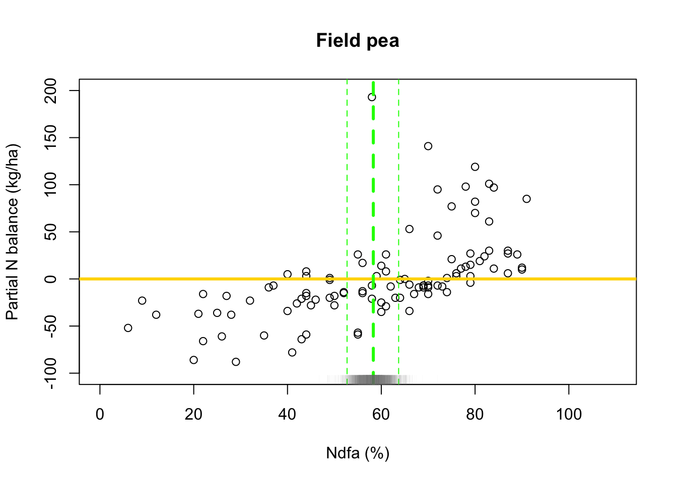

1.8 Low information content data

What value of Ndfa is needed to achieve a neutral N balance?

df.wl <- df.all[which(df.all$Scenario=="Scenario B"),]
plot(df.wl$Ndfa,df.wl$PartNbalance,
 xlab="Ndfa (%)",ylab="Partial N balance (kg/ha)",
 xlim=c(0,110),ylim=c(-100,200),main="White lupin")
abline(a=0,b=0,col="gold",lwd=3)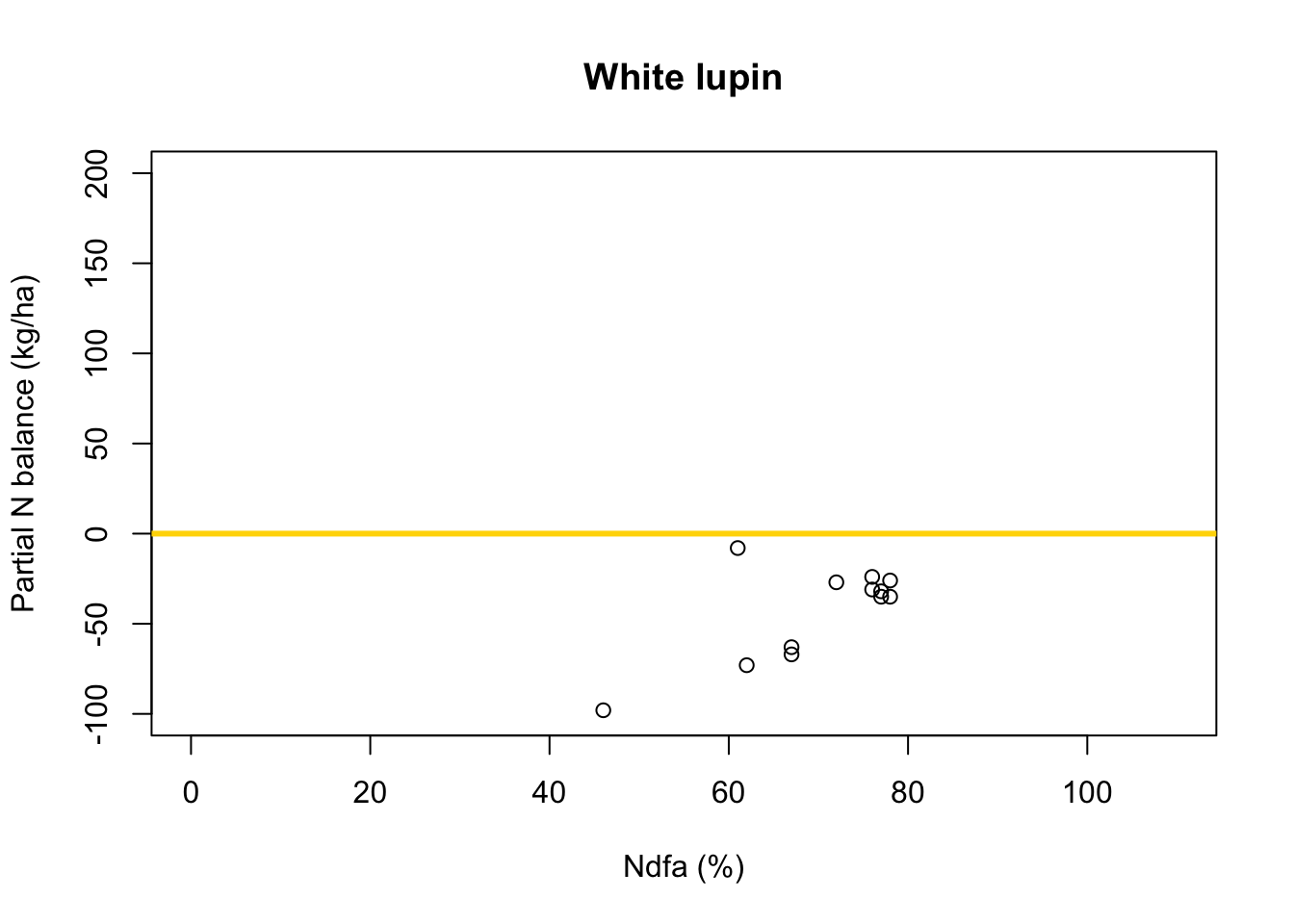

Using least squares

m1 <- lm(PartNbalance ~ Ndfa,data=df.wl)

What value of Ndfa is needed to achieve a neutral N balance?

beta0.hat <- as.numeric(coef(m1)[1])
beta1.hat <- as.numeric(coef(m1)[2])
theta.hat <- -beta0.hat/beta1.hat
theta.hat

## [1] 93.09456

Visual representation of $\theta$

# Plot data, line of best fit and theta 
plot(df.wl$Ndfa,df.wl$PartNbalance,
 xlab="Ndfa (%)",ylab="Partial N balance (kg/ha)",
 xlim=c(0,110),ylim=c(-100,200),main="White lupin")
abline(a=0,b=0,col="gold",lwd=3)
abline(m1,col="red",lwd=3)
abline(v=93.1,lwd=3,lty=2,col="green")

Using likelihood-based inference

Fit linear model to data using using maximum likelihood estimation

library(nlme)
# Fit simple linear regression model using maximum likelihood estimation
m2 <- gls(PartNbalance ~ Ndfa,data=df.wl,method="ML")

What value of Ndfa is needed to achieve a neutral N balance?

# Use maximum likelihood estimate (MLE) to obtain estimate of theta
beta0.hat <- as.numeric(coef(m2)[1])
beta1.hat <- as.numeric(coef(m2)[2])
theta.hat <- -beta0.hat/beta1.hat
theta.hat

## [1] 93.09456

# Use delta method to obtain approximate approximate standard errors and
# then construct Wald-type confidence intervals
library(msm)
theta.se <- deltamethod(~-x1/x2, mean=coef(m2), cov=vcov(m2))

theta.ci <- c(theta.hat-1.96*theta.se,theta.hat+1.96*theta.se)
theta.ci

## [1]  76.91135 109.27778

Visual representation of $\theta$

# Plot data, line of best fit and theta 
plot(df.wl$Ndfa,df.wl$PartNbalance,
 xlab="Ndfa (%)",ylab="Partial N balance (kg/ha)",
 xlim=c(0,110),ylim=c(-100,200),main="White lupin")
abline(a=0,b=0,col="gold",lwd=3)
abline(m1,col="red",lwd=3)
abline(v=93.1,lwd=3,lty=2,col="green") 
abline(v=76.9,lwd=1,lty=2,col="green") 
abline(v=109.2,lwd=1,lty=2,col="green")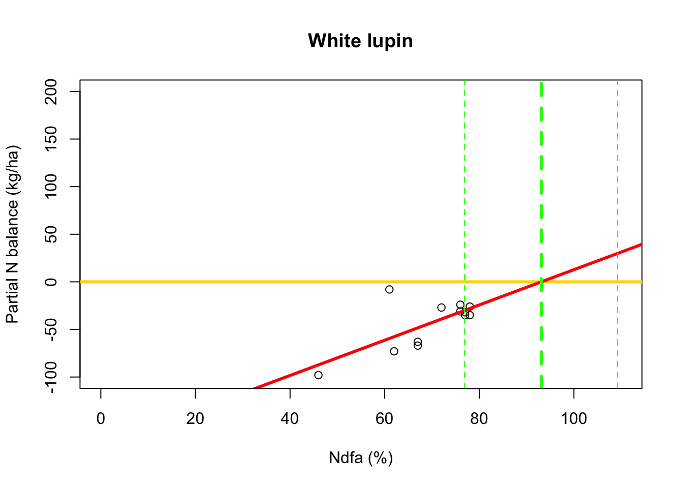

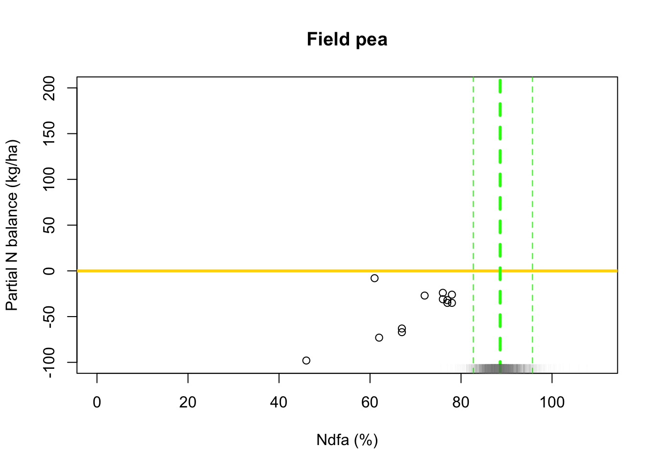
Using Bayesian inference

Assume that $y_i=\beta_{0}+\beta_{1}x_{i}+\varepsilon_i$ with $\varepsilon_i\sim \text{N}(0,\sigma^2)$ , $\beta_{0}\sim \text{N}(0,10^6)$ and $\beta_{1}\sim \text{N}(2.5,0.1)$
Model fitting

samples <- norm.reg.mcmc(y = df.wl$PartNbalance,X = model.matrix(~ Ndfa,data=df.wl),
                      beta.mn = c(0,2.5),beta.var=c(10^6,0.1),
                      s2.mn = 10, s2.sd = 10^6,
                      n.mcmc = 5000)

burn.in <- 1000
# Look a histograms of posterior distributions
par(mfrow=c(2,1),mar=c(5,6,1,1))
hist(samples$beta.save[1,-c(1:1000)],xlab=expression(beta[0]*"|"*bold(y)),ylab=expression("["*beta[0]*"|"*bold(y)*"]"),freq=FALSE,col="grey",main="",breaks=30)
hist(samples$beta.save[2,-c(1:1000)],xlab=expression(beta[1]*"|"*bold(y)),ylab=expression("["*beta[1]*"|"*bold(y)*"]"),freq=FALSE,col="grey",main="",breaks=30)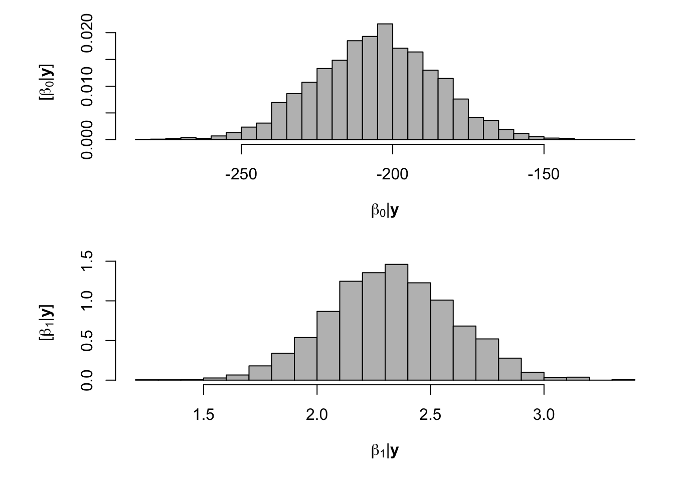

What value of Ndfa is needed to achieve a neutral N balance?

hist(-samples$beta.save[1,-c(1:1000)]/samples$beta.save[2,-c(1:1000)],xlab=expression(theta*"|"*bold(y)),ylab=expression("["*theta*"|"*bold(y)*"]"),freq=FALSE,col="grey",main="",breaks=30)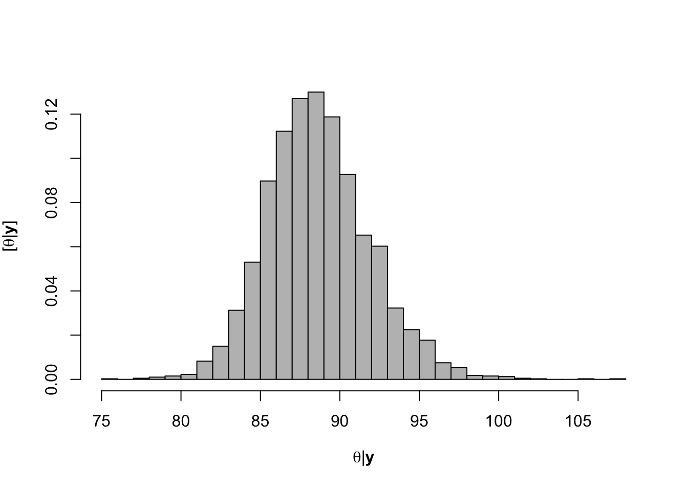

# Expected value (mean) of theta        
mean(-samples$beta.save[1,]/samples$beta.save[2,])

## [1] 88.63508

# 95% credible intervals for theta
quantile(-samples$beta.save[1,]/samples$beta.save[2,],prob=c(0.025,0.975))

##     2.5%    97.5% 
## 83.01900 95.53826

# Plot data and theta 
plot(df.wl$Ndfa,df.wl$PartNbalance,
 xlab="Ndfa (%)",ylab="Partial N balance (kg/ha)",
 xlim=c(0,110),ylim=c(-100,200),main="Field pea")
abline(a=0,b=0,col="gold",lwd=3)
abline(v=88.6,lwd=3,lty=2,col="green") 
abline(v=82.7,lwd=1,lty=2,col="green") 
abline(v=95.7,lwd=1,lty=2,col="green") 
rug(-samples$beta.save[1,]/samples$beta.save[2,],col=gray(0.5,0.03))