14 Day 14 (March 6)
14.1 Announcements
Update on projects
Read Chs. 11 and 12
Selected questions/clarifications from journals
- Didn’t have time to do this :(
14.2 The Bayesian Linear Model
- Example revisiting white lupine data set from day 1
- Details of data and analysis from Palmero et al. (2024)
- Live example
14.3 Bayesian prediction
Prior prediction vs. posterior prediction
- Prior prediction is used before fitting your model to data. It is used as a model checking tool (e.g., to see if priors are reasonable) or to do prediction if you have little or no data.
- Posterior prediction is more typically what you think of as prediction. It is done after fitting your model to data.
Prior prediction of disease spread (here)
Prior prediction example: my retirement
- Personal information
- Obviously this isn’t my actual information, but it isn’t too far off!
- Since I am a millennial/doge I don’t think social security will be around when I retire (i.e., assume social security contributes $0 to my retirement)
- As of 1/1/25 I have $250,000 in 401k retirement in accounts
- All of money is invested into an S&P 500 index fund (VOO to be exact)
- I am 38 as of 1/1/25
- I will contribute ~ $20k to my retirement each year
- I want to know how much pre-tax money I will have at a given retirement age (e.g., 60, 65, 70, etc)
- Example using a mathematical model
- Whiteboard demonstration
- What are the model assumptions?
- In program R
# The value of my 401k retirement account as of 1/1/25
y_2025 <- 250000


# How much money will I add to my 401k each year
q <- 20000


# Rate of return for S&P 500 index fund
r <- 0.12


# How much $ will I have in 2026
y_2026 <- y_2025*(1+r)+q
y_2026
## [1] 3e+05## [1] 356000## [1] 418720# Using a for loop to calculate how much $ will I have year <- seq(2025,2025+22,by=1) y <- matrix(,length(year),1) rownames(y) <- year y[1,1] <- 250000 for(t in 1:22){ y[t+1,1] <- y[t,1]*(1+r)+q } plot(year,y/10^6,typ="b",pch=20,col="deepskyblue",xlab="Year",ylab="Pretax retirement amount ($ millions)")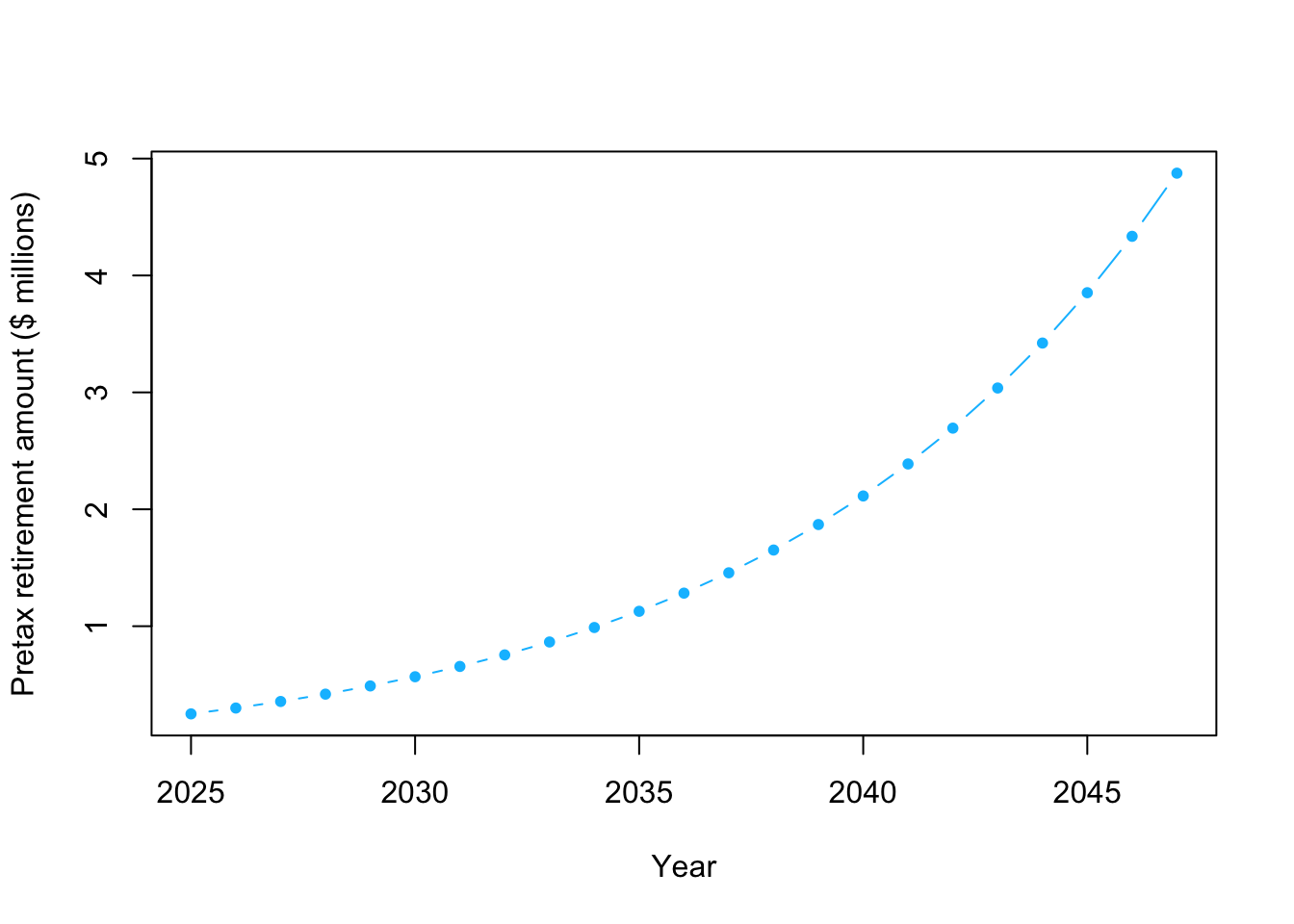
# How much $ will I have when I am 60?
# Note that units are millions of $
retirement.year <- 2025+22
y[which(year==retirement.year)]/10^6
## [1] 4.875129- Example using a Bayesian statistical model
- Whiteboard demonstration
- S&P 500 return since inception in 1957
# Download S&P 500 returns
url <- "https://www.dropbox.com/s/81ccahyuaas1zpd/s%26p500.csv?dl=1"
df.sp500 <- read.csv(url)

head(df.sp500)
## year return ## 1 2022 -0.1811 ## 2 2021 0.2871 ## 3 2020 0.1840 ## 4 2019 0.3149 ## 5 2018 -0.0438 ## 6 2017 0.2183## [1] 0.1152742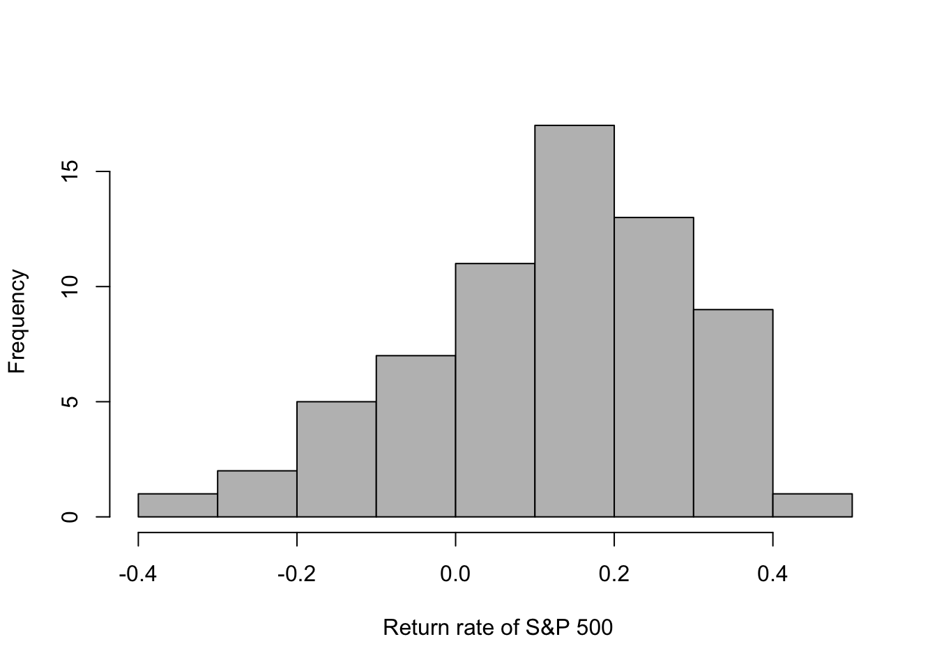 - Example using the prior predictive distribution
- Personal information
# Download S&P 500 returns
url <- "https://www.dropbox.com/s/81ccahyuaas1zpd/s%26p500.csv?dl=1"
df.sp500 <- read.csv(url)

# The value of my 401k retirement account as of 1/1/25
y_2025 <- 250000

# How much money will I add to my 401k each year
q <- 20000


# Using a for loop to calculate how much $ will I have
year <- seq(2025,2025+22,by=1)
Y <- matrix(,length(year),1000)
rownames(Y) <- year
Y[1,] <- y_2025

set.seed(3410)
for(m in 1:1000){
for(t in 1:22){
  r <- sample(df.sp500$return,1)
  Y[t+1,m] <- Y[t,m]*(1+r)+q
              }
                }


# Prior predictive distribution for a given year
retirement.year <- 2025+22
hist(Y[which(year==retirement.year),]/10^6,col="grey",freq=FALSE,xlab="Pretax retirement amount ($ millions)",main="")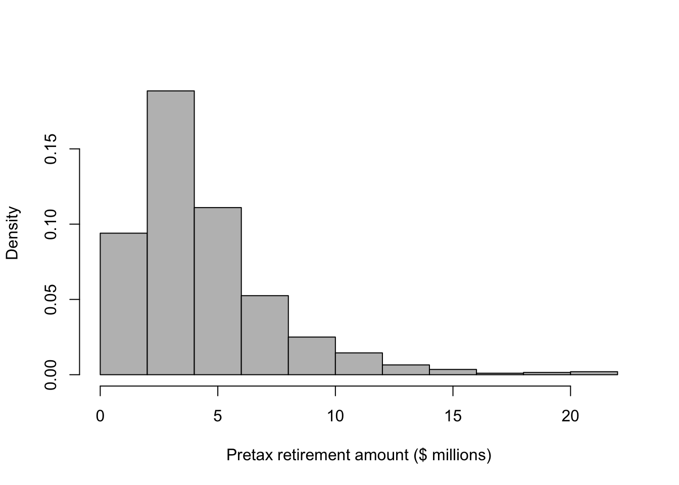
## [1] 4.393178## [1] 21.66186## [1] 0.3341111## 2.5% 97.5%
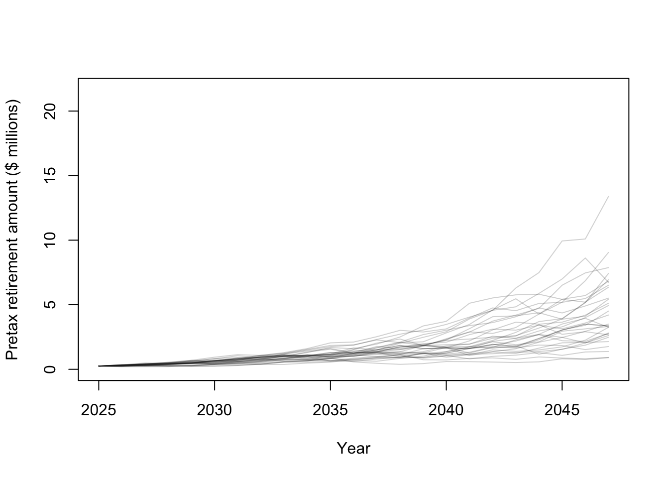
## 0.901447 12.309287# Plot some financial trajectories (i.e., random draws from the prior predictive distribution)
plot(year,Y[,1]/10^6,typ="l",lwd=1,ylim=c(0,max(Y/10^6)),col=rgb(0.1,0.1,0.1,.2),xlab="Year",ylab="Pretax retirement amount ($ millions)")
for(i in 1:30){
points(year,Y[,i]/10^6,typ="l",lwd=1,col=rgb(0.1,0.1,0.1,.2))
}
# Plot of prior predictive distribution for all years
E.Y <- apply(Y/10^6,1,mean)
u.CI <- apply(Y/10^6,1,quantile,prob=0.975)
l.CI <- apply(Y/10^6,1,quantile,prob=0.025)
max.Y <- apply(Y/10^6,1,max)
min.Y <- apply(Y/10^6,1,min)

plot(year,E.Y,typ="l",lwd=3,ylim=c(0,max(max.Y)),xlab="Year",ylab="Pretax retirement amount ($ millions)")
points(year,max.Y,typ="l",lwd=3,col="red")
points(year,min.Y,typ="l",lwd=3,col="red")
polygon(c(year,rev(year)),c(u.CI,rev(l.CI)),
        col=rgb(0.5,0.5,0.5,0.5),border=rgb(0.5,0.5,0.5,0.5))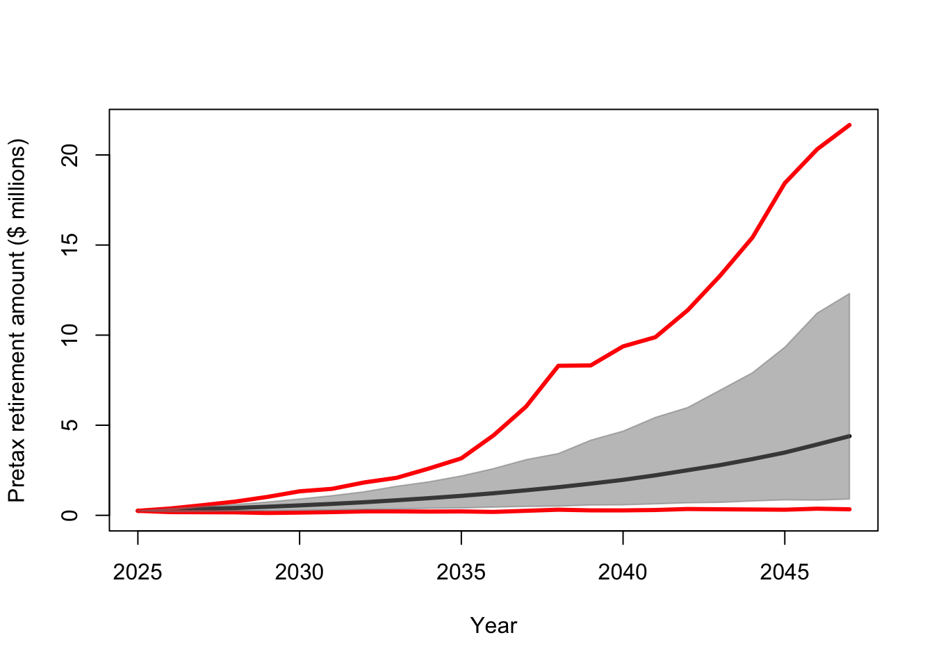
- Example revisiting white lupine data set from day 1
- Details of data and analysis from Palmero et al. (2024)
- Live example