4 Day 4 (June 6)

4.1 Announcements

• Tutoring for program R

  • Dickens Hall room 108
  • 12:30 - 1:30 Monday - Friday

• Recommended reading

  • Chapters 1 and 2 (pgs 1 - 28) in Linear Models with R
  • Chapter 2 in Applied Regression and ANOVA Using SAS

• Final project is posted

• Assignment 2 is posted a due Wednesday June 12

• Special in-class event on Friday!

4.2 Introduction to linear models

• What is a model?

• What is a linear model?

  • Most widely used model in science, engineering, and statistics

  • Vector form: $\mathbf{y}=\beta_{0}+\beta_{1}\mathbf{x}_{1}+\beta_{2}\mathbf{x}_{2}+\ldots+\beta_{p}\mathbf{x}_{p}+\boldsymbol{\varepsilon}$

  • Matrix form: $\mathbf{y}=\mathbf{X}\boldsymbol{\beta}+\boldsymbol{\varepsilon}$

  • Which part of the model is the mathematical model

  • Which part of the model makes the linear model a “statistical” model

  • Visual

• Which of the four below are a linear model $$\mathbf{y}=\beta_{0}+\beta_{1}\mathbf{x}_{1}+\beta_{2}\mathbf{x}^{2}_{1}+\boldsymbol{\varepsilon}$$ $$\mathbf{y}=\beta_{0}+\beta_{1}\mathbf{x}_{1}+\beta_{2}\text{log(}\mathbf{x}_{1}\text{)}+\boldsymbol{\varepsilon}$$ $$\mathbf{y}=\beta_{0}+\beta_{1}e^{\beta_{2}\mathbf{x}_{1}}+\boldsymbol{\varepsilon}$$ $$\mathbf{y}=\beta_{0}+\beta_{1}\mathbf{x}_{1}+\text{log(}\beta_{2}\text{)}\mathbf{x}_{1}+\boldsymbol{\varepsilon}$$

• Why study the linear model?

  • Building block for more complex models (e.g., GLMs, mixed models, machine learning, etc)
  • We know the most about it

4.3 Estimation

• Three options to estimate $\boldsymbol{\beta}$
  • Minimize a loss function
  • Maximize a likelihood function
  • Find the posterior distribution
  • Each option requires different assumptions

4.4 Loss function approach

• Define a measure of discrepancy between the data and the mathematical model
  • Find the values of $\boldsymbol{\beta}$ that make $\mathbf{X}\boldsymbol{\beta}$ “closest” to $\mathbf{y}$
  • Visual
• Classic example $$\underset{\boldsymbol{\beta}}{\operatorname{argmin}}\sum_{i=1}^{n}(y_i-\mathbf{x}_{i}^{\prime}\boldsymbol{\beta})^2$$ or in matrix form $$\underset{\boldsymbol{\beta}}{\operatorname{argmin}}(\mathbf{y} - \mathbf{X}\boldsymbol{\beta})^{\prime}(\mathbf{y} - \mathbf{X}\boldsymbol{\beta})$$ which results in $$\hat{\boldsymbol{\beta}}=(\mathbf{X}^{\prime}\mathbf{X})^{-1}\mathbf{X}^{\prime}\mathbf{y}$$
• Three ways to do it in program R
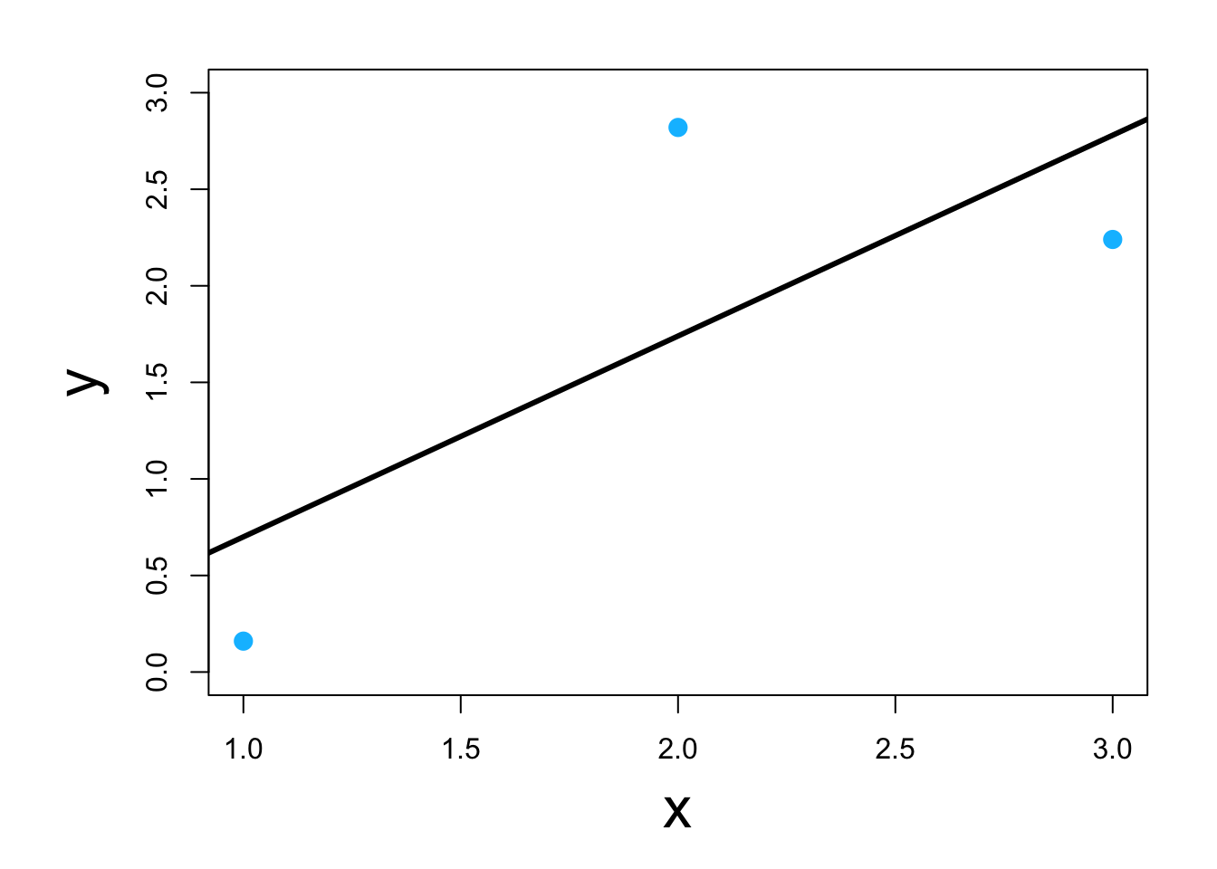
  • Using scalar calculus and algebra (kind of)

  y <- c(0.16,2.82,2.24)
  x <- c(1,2,3)
  
  y.bar <- mean(y)
  x.bar <- mean(x)
  
  # Estimate the slope parameter
  beta1.hat <- sum((x-x.bar)*(y-y.bar))/sum((x-x.bar)^2)
  beta1.hat

  ## [1] 1.04

  # Estimate the intercept parameter
  beta0.hat <- y.bar - sum((x-x.bar)*(y-y.bar))/sum((x-x.bar)^2)*x.bar
  beta0.hat

  ## [1] -0.34