35 Day 34 (July 24)
35.1 Announcements
- Teval
- Final grades
- More about challenger example here
35.2 Transformations of the response
Big picture idea
- Select a function that transforms \(\mathbf{y}\) such that the assumptions of normality are approximately correct.
Two cultures
- This is with respect to \(\mathbf{y}\) and not the predictors. Transforming the predictors is not at all controversial.
- Trade offs
- Difficult to apply sometimes (e.g., \(\text{log(}\mathbf{y}+c)\) for count data)
- Difficult to interpret on the transformed scale
- If normality is an appropriate assumption, we can use the general linear model \(\textbf{y}\sim\text{N}(\mathbf{X}\boldsymbol{\beta},\mathbf{V})\)
Example
- Number of whooping cranes each year
url <- "https://www.dropbox.com/s/ihs3as87oaxvmhq/Butler%20et%20al.%20Table%201.csv?dl=1"
df1 <- read.csv(url)
plot(df1$Winter,df1$N,typ="b",xlab="Year",ylab="Population Size",ylim=c(0,300),lwd=1.5,pch="*")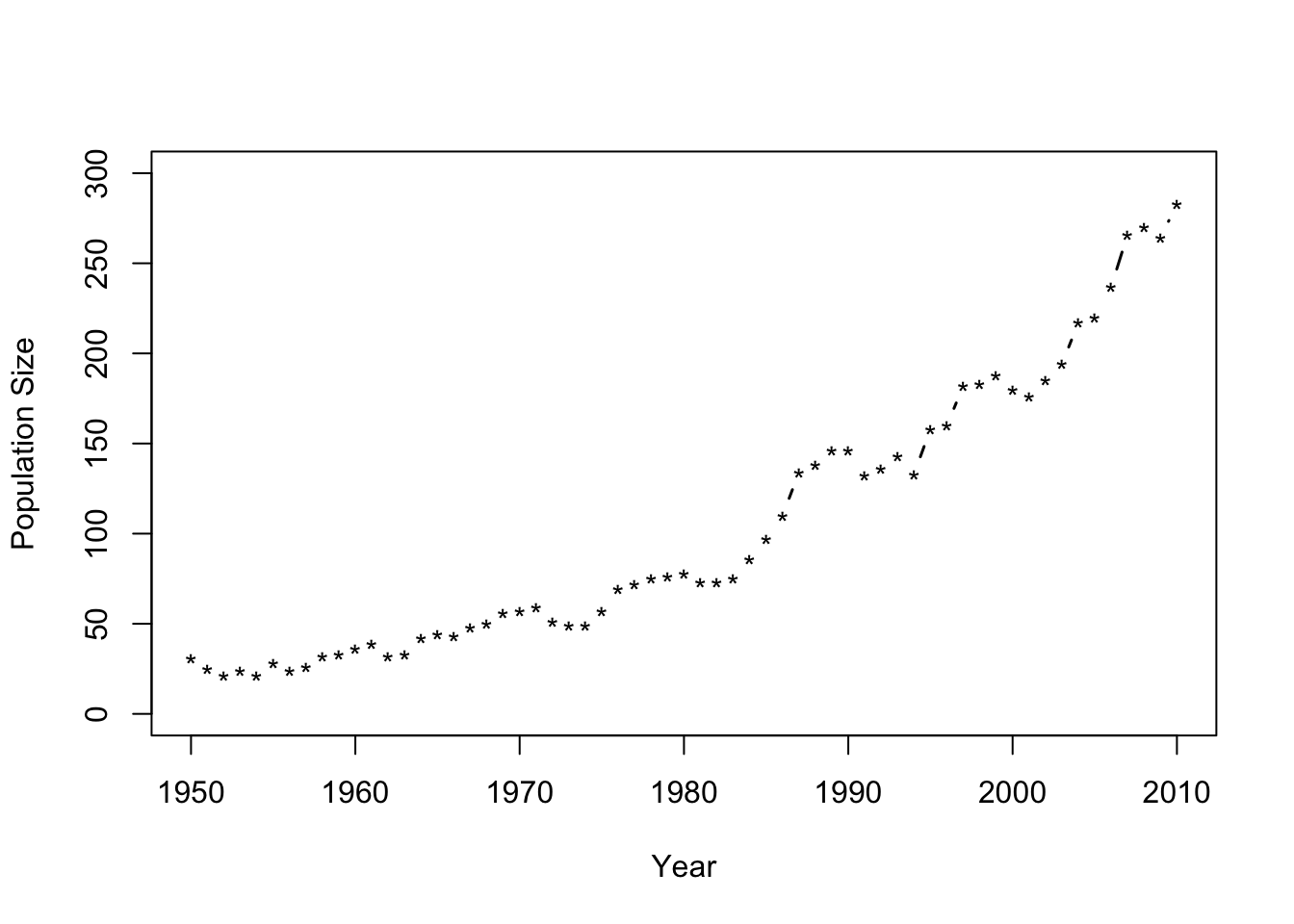
- Fit the model \(\mathbf{y}=\beta_{0}+\beta_{1}\mathbf{x}+\boldsymbol{\varepsilon}\) where \(\boldsymbol{\varepsilon}\sim\text{N}(\mathbf{0},\sigma^{2}\mathbf{I})\) and \(\mathbf{x}\) is the year.
m1 <- lm(N~Winter,data=df1)
plot(df1$Winter,df1$N,typ="b",xlab="Year",ylab="Population Size",ylim=c(0,300),lwd=1.5,pch="*")
abline(m1,col="gold")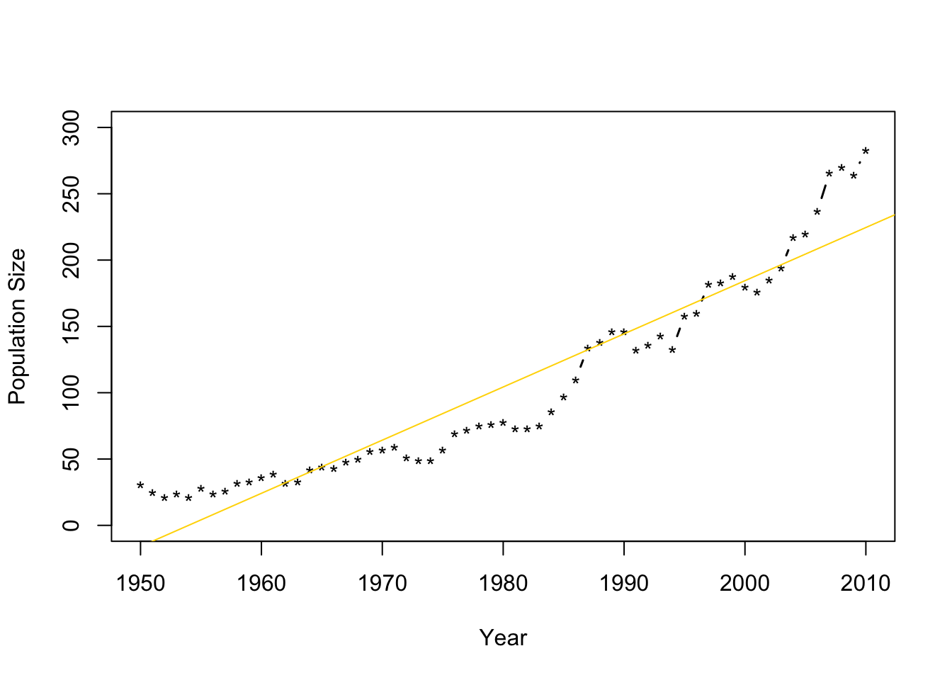
- Check model assumptions
e.hat <- residuals(m1)

#Check normality
hist(e.hat,col="grey",breaks=10,main="",xlab=expression(hat(epsilon)))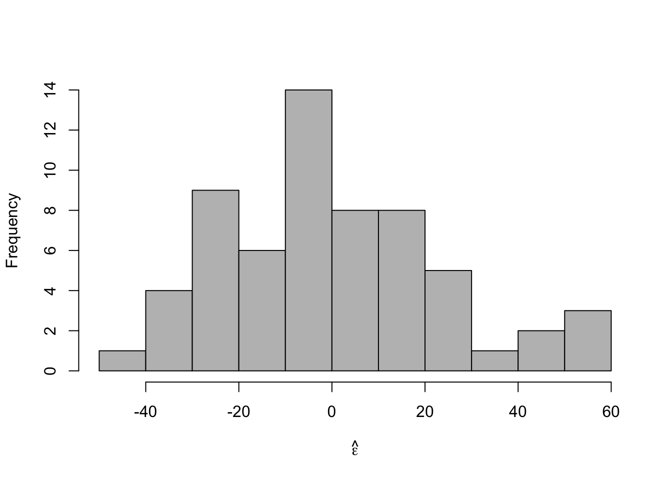
##
##  Shapiro-Wilk normality test
##
## data:  e.hat
## W = 0.96653, p-value = 0.09347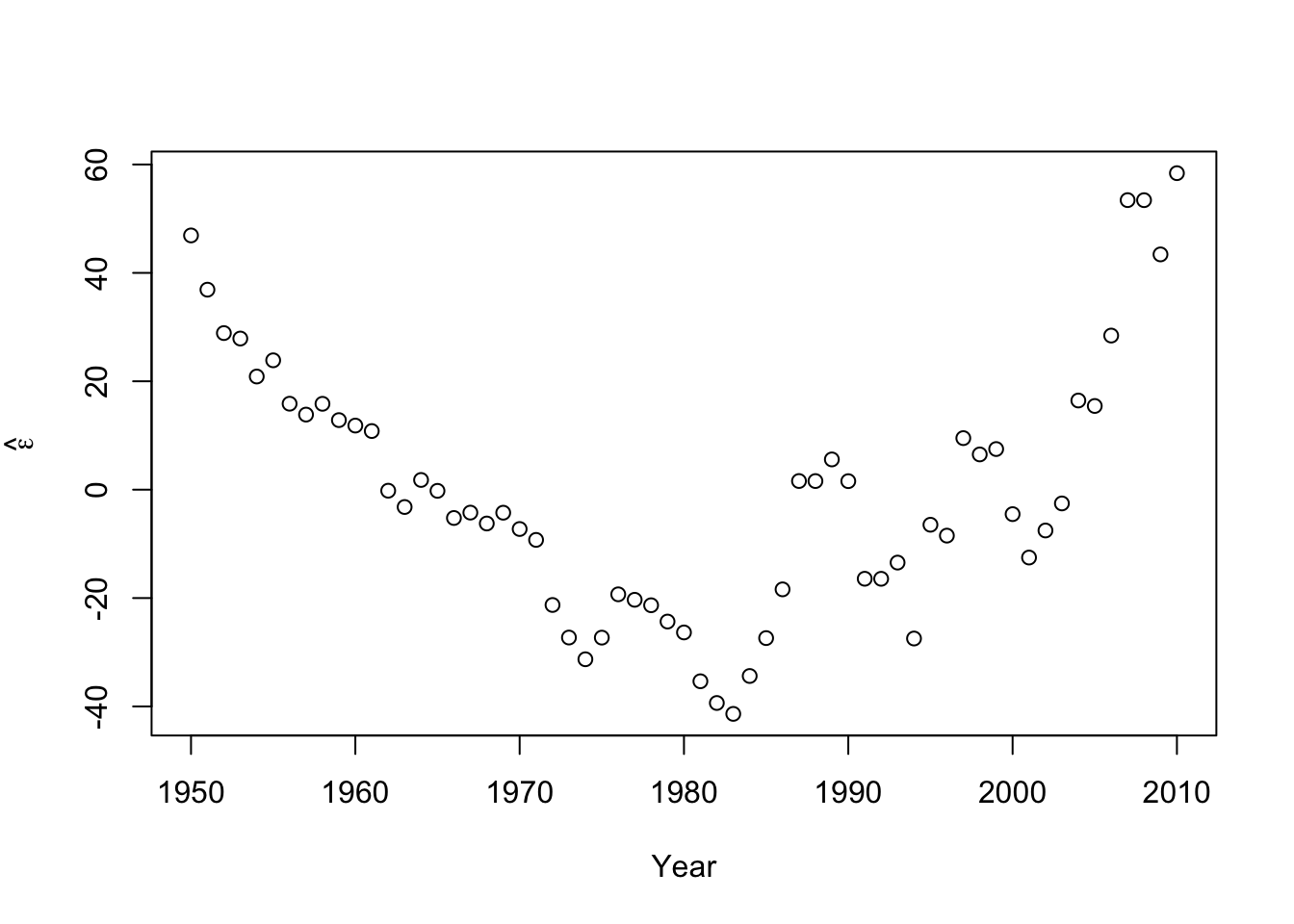
#Check for autocorrelation among residuals
plot(e.hat[1:60],e.hat[2:61],xlab=expression(hat(epsilon)[t]),ylab=expression(hat(epsilon)[t+1]))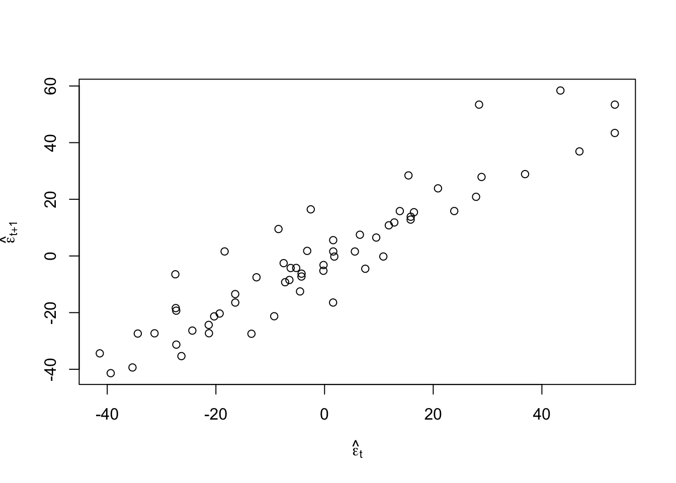
## [1] 0.9273559## ## Durbin-Watson test ## ## data: m1 ## DW = 0.13355, p-value < 2.2e-16 ## alternative hypothesis: true autocorrelation is greater than 0- Log transformation (i.e., \(\text{log}(\mathbf{y})\)).
- \(\text{log}(\mathbf{y})=\beta_{0}+\beta_{1}\mathbf{x}+\boldsymbol{\varepsilon}\) where \(\boldsymbol{\varepsilon}\sim\text{N}(\mathbf{0},\sigma^{2}\mathbf{I})\) and \(\mathbf{x}\) is the year.
- What model is implied by this transformation?
- If \(z\sim\text{N}(\mu,\sigma^{2})\), then \(\text{E}(e^{z})=e^{\mu+\frac{\sigma^{2}}{2}}\) and \(\text{Var}(e^{z})=(e^{\sigma^{2}}-1)e^{2\mu+\sigma^{2}}\)
- Fit the model
m2 <- lm(log(N)~Winter,data=df1) plot(df1$Winter,df1$N,typ="b",xlab="Year",ylab="Population Size",ylim=c(0,300),lwd=1.5,pch="*") abline(m1,col="gold") ev.y.hat <- exp(predict(m2)) # Possible because of invariance property of MLEs points(df1$Winter,ev.y.hat,typ="l",col="deepskyblue")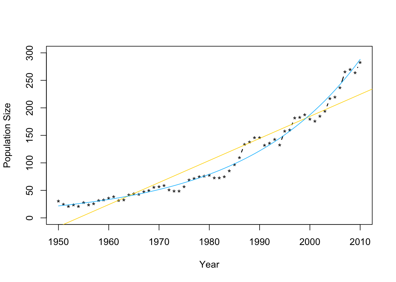 - Check model assumptions
e.hat <- residuals(m2)

#Check normality
hist(e.hat,col="grey",breaks=10,main="",xlab=expression(hat(epsilon)))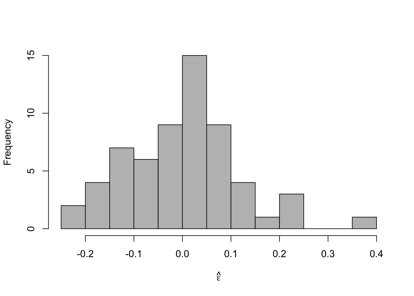
## ## Shapiro-Wilk normality test ## ## data: e.hat ## W = 0.97059, p-value = 0.1489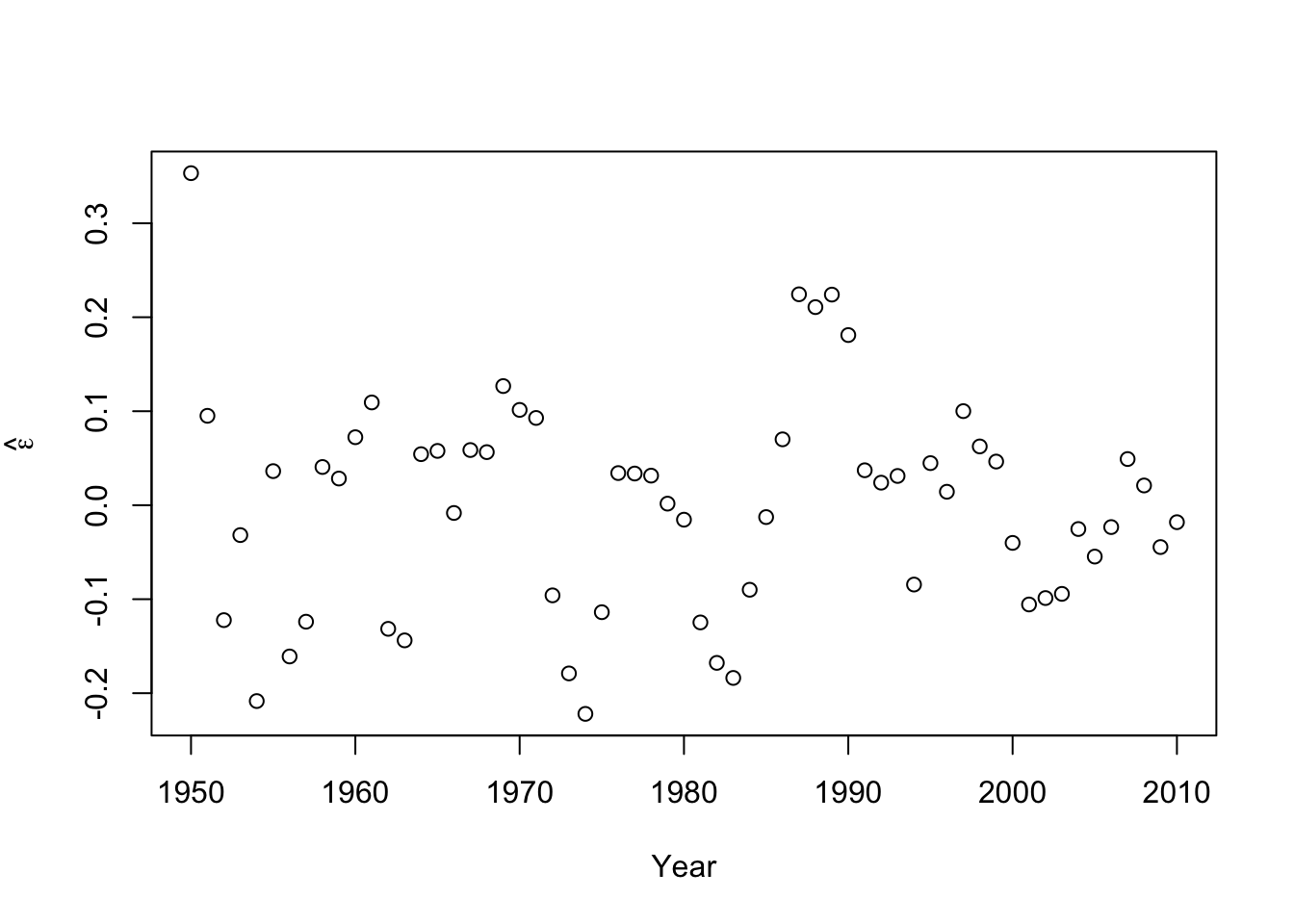 - Confidence intervals and prediction intervals
plot(df1$Winter,df1$N,typ="b",xlab="Year",ylab="Population Size",ylim=c(0,300),lwd=1.5,pch="*")
ev.y.hat <- exp(predict(m2)) # Possible because of invariance property of MLEs
points(df1$Winter,ev.y.hat,typ="l",col="deepskyblue")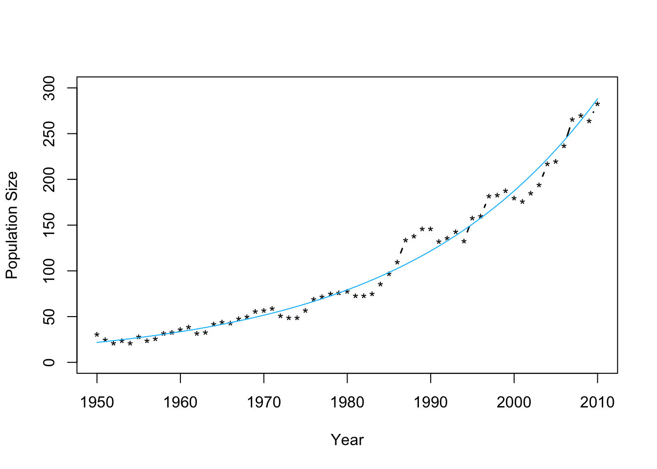
## fit lwr upr ## 1 3.080718 3.0223 3.139136## fit lwr upr ## 1 3.080718 2.842504 3.318933
35.3 Bayesian linear model
Assume that \(y_i=\beta_{0}+\beta_{1}x_{i}+\varepsilon_i\) with \(\varepsilon_i\sim \text{N}(0,\sigma^2)\), \(\beta_{0}\sim \text{N}(0,10^6)\) and \(\beta_{1}\sim \text{N}(0,10^6)\)
Statistical inference
- Using Bayes rule (Bayes 1763) we can obtain the joint posterior distribution
\[[\beta_0,\beta_1,\sigma_{\varepsilon}^{2}|\mathbf{y}]=\frac{[\mathbf{y}|\beta_0,\beta_1,\sigma_{\varepsilon}^{2}][\beta_0][\beta_1][\sigma_{\varepsilon}^{2}]}{\int\int\int [\mathbf{y}|\beta_0,\beta_1,\sigma_{\varepsilon}^{2}][\beta_0][\beta_1][\sigma_{\varepsilon}^{2}]d\beta_0d\beta_1,d\sigma_{\varepsilon}^{2}}\]
- Statistical inference about a paramters is obtained from the marginal posterior distributions \[[\beta_0|\mathbf{y}]=\int[\beta_0,\beta_1,\sigma_{\varepsilon}^{2}|\mathbf{y}]d\beta_1d\sigma_{\varepsilon}^{2}\] \[[\beta_1|\mathbf{y}]=\int[\beta_0,\beta_1,\sigma_{\varepsilon}^{2}|\mathbf{y}]d\beta_0d\sigma_{\varepsilon}^{2}\] \[[\sigma_{\varepsilon}^{2}|\mathbf{y}]=\int[\beta_0,\beta_1,\sigma_{\varepsilon}^{2}|\mathbf{y}]d\beta_0d\beta_1\]
- Derived quantities can be obtained by transformations of the joint posterior
- Using Bayes rule (Bayes 1763) we can obtain the joint posterior distribution
\[[\beta_0,\beta_1,\sigma_{\varepsilon}^{2}|\mathbf{y}]=\frac{[\mathbf{y}|\beta_0,\beta_1,\sigma_{\varepsilon}^{2}][\beta_0][\beta_1][\sigma_{\varepsilon}^{2}]}{\int\int\int [\mathbf{y}|\beta_0,\beta_1,\sigma_{\varepsilon}^{2}][\beta_0][\beta_1][\sigma_{\varepsilon}^{2}]d\beta_0d\beta_1,d\sigma_{\varepsilon}^{2}}\]
Computations
- Using a Markov chain Monte Carlo algorithm (see Ch.11 in Hooten and Hefley 2019)
norm.reg.mcmc <- function(y,X,beta.mn,beta.var,s2.mn,s2.sd,n.mcmc){

  #
  #  Code Box 11.1
  #

  ###
  ### Subroutines
  ###

  library(mvtnorm)

  invgammastrt <- function(igmn,igvar){
q <- 2+(igmn^2)/igvar
r <- 1/(igmn*(q-1))
list(r=r,q=q)
  }

  invgammamnvr <- function(r,q){  #  This fcn is not necessary
mn <- 1/(r*(q-1))
vr <- 1/((r^2)*((q-1)^2)*(q-2))
list(mn=mn,vr=vr)
  }

  ###
  ### Hyperpriors
  ###

  n=dim(X)[1]
  p=dim(X)[2]
  r=invgammastrt(s2.mn,s2.sd^2)$r
  q=invgammastrt(s2.mn,s2.sd^2)$q
  Sig.beta.inv=diag(p)/beta.var

  beta.save=matrix(0,p,n.mcmc)
  s2.save=rep(0,n.mcmc)
  Dbar.save=rep(0,n.mcmc)
  y.pred.mn=rep(0,n)

  ###
  ### Starting Values
  ###

  beta=solve(t(X)%*%X)%*%t(X)%*%y

  ###
  ### MCMC Loop
  ###

  for(k in 1:n.mcmc){


###
### Sample s2
###

tmp.r=(1/r+.5*t(y-X%*%beta)%*%(y-X%*%beta))^(-1)
tmp.q=n/2+q

s2=1/rgamma(1,tmp.q,,tmp.r)

###
### Sample beta
###

tmp.var=solve(t(X)%*%X/s2 + Sig.beta.inv)
tmp.mn=tmp.var%*%(t(X)%*%y/s2 + Sig.beta.inv%*%beta.mn)

beta=as.vector(rmvnorm(1,tmp.mn,tmp.var,method="chol"))

###
### Save Samples
###

beta.save[,k]=beta
s2.save[k]=s2

  }

  ###
  ###  Write Output
  ###

  list(beta.save=beta.save,s2.save=s2.save,y=y,X=X,n.mcmc=n.mcmc,n=n,r=r,q=q,p=p)

}
Model fitting
- MCMC
# Preliminary steps
url <- "https://www.dropbox.com/scl/fi/nr1deg9v53wyclgsjkddm/Fig3_data.csv?rlkey=iqrmjmwhtv1xha2kviq0fjrln&dl=1"
df.all <- read.csv(url)
df.fp <- df.all[which(df.all$Scenario=="Scenario A"),]

samples <- norm.reg.mcmc(y = df.fp$PartNbalance,X = model.matrix(~ Ndfa,data=df.fp),
                      beta.mn = c(0,0),beta.var=c(10^6,10^6),
                      s2.mn = 10, s2.sd = 10^6,
                      n.mcmc = 5000)

burn.in <- 1000
# Look a histograms of posterior distributions
par(mfrow=c(2,1),mar=c(5,6,1,1))
hist(samples$beta.save[1,-c(1:1000)],xlab=expression(beta[0]*"|"*bold(y)),ylab=expression("["*beta[0]*"|"*bold(y)*"]"),freq=FALSE,col="grey",main="",breaks=30)
hist(samples$beta.save[2,-c(1:1000)],xlab=expression(beta[1]*"|"*bold(y)),ylab=expression("["*beta[1]*"|"*bold(y)*"]"),freq=FALSE,col="grey",main="",breaks=30)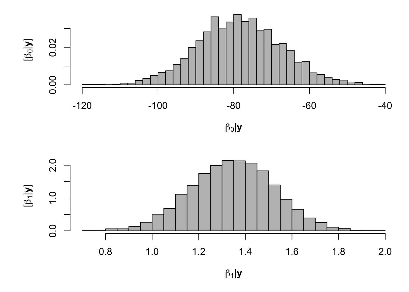
What value of Ndfa is needed to achieve a neutral N balance?
hist(-samples$beta.save[1,-c(1:1000)]/samples$beta.save[2,-c(1:1000)],xlab=expression(theta*"|"*bold(y)),ylab=expression("["*theta*"|"*bold(y)*"]"),freq=FALSE,col="grey",main="",breaks=30)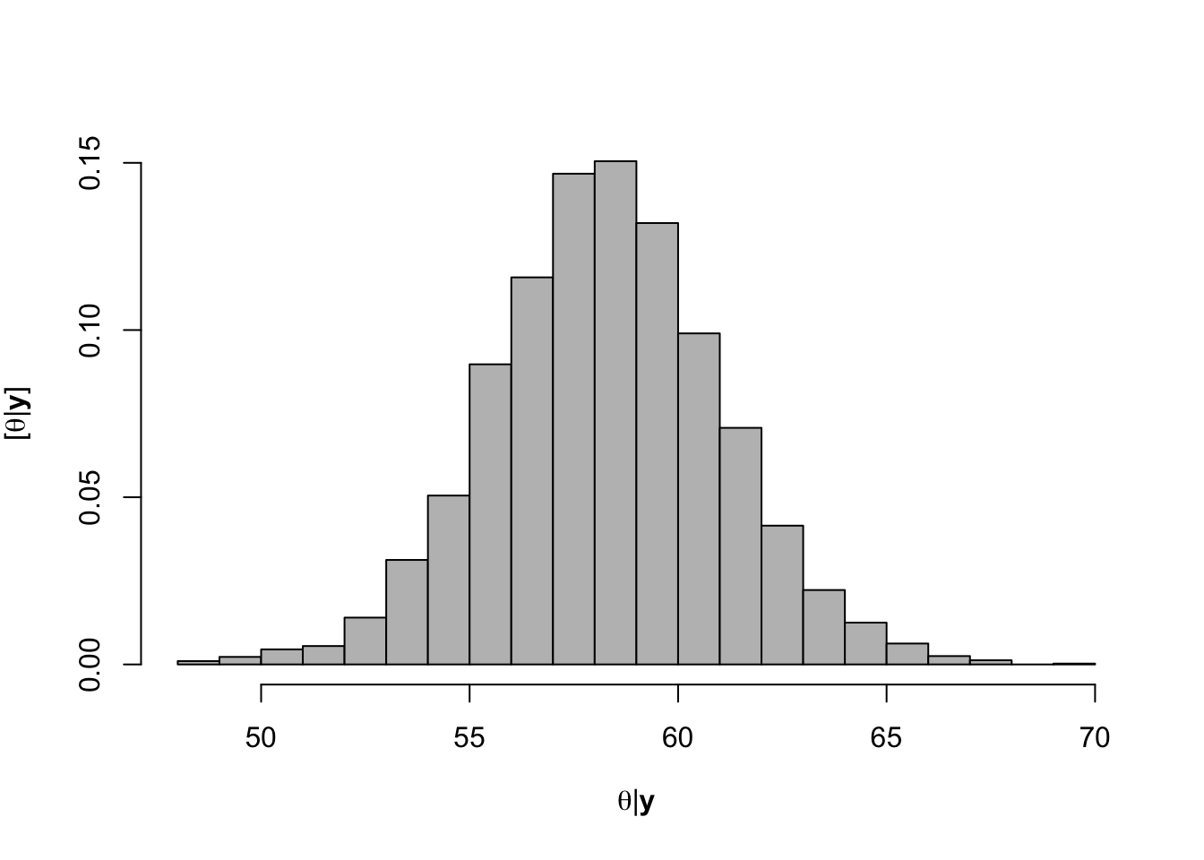
## [1] 58.26407# 95% credible intervals for theta quantile(-samples$beta.save[1,]/samples$beta.save[2,],prob=c(0.025,0.975))## 2.5% 97.5% ## 52.78771 63.79724- Visual representation of posterior distribuiton of theta \(\theta\)
# Plot data and theta
plot(df.fp$Ndfa,df.fp$PartNbalance,
 xlab="Ndfa (%)",ylab="Partial N balance (kg/ha)",
 xlim=c(0,110),ylim=c(-100,200),main="Field pea")
abline(a=0,b=0,col="gold",lwd=3)
abline(v=58.3,lwd=3,lty=2,col="green")
abline(v=52.7,lwd=1,lty=2,col="green")
abline(v=63.7,lwd=1,lty=2,col="green")
rug(-samples$beta.save[1,]/samples$beta.save[2,],col=gray(0.5,0.03))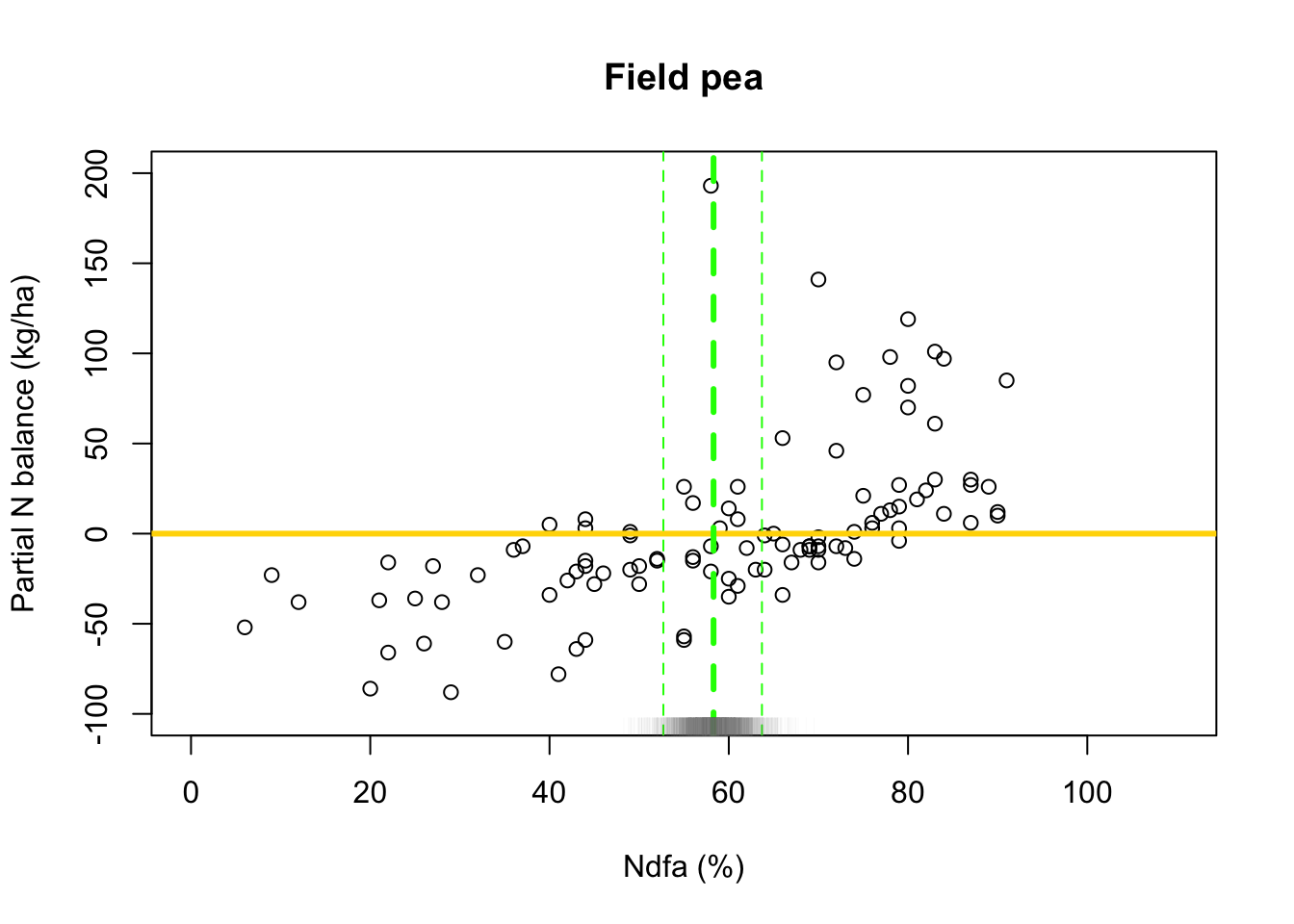
Exercise
- What value of Ndfa is needed to achieve a neutral N balance?
df.wl <- df.all[which(df.all$Scenario=="Scenario B"),]
plot(df.wl$Ndfa,df.wl$PartNbalance,
 xlab="Ndfa (%)",ylab="Partial N balance (kg/ha)",
 xlim=c(0,110),ylim=c(-100,200),main="White lupin")
abline(a=0,b=0,col="gold",lwd=3)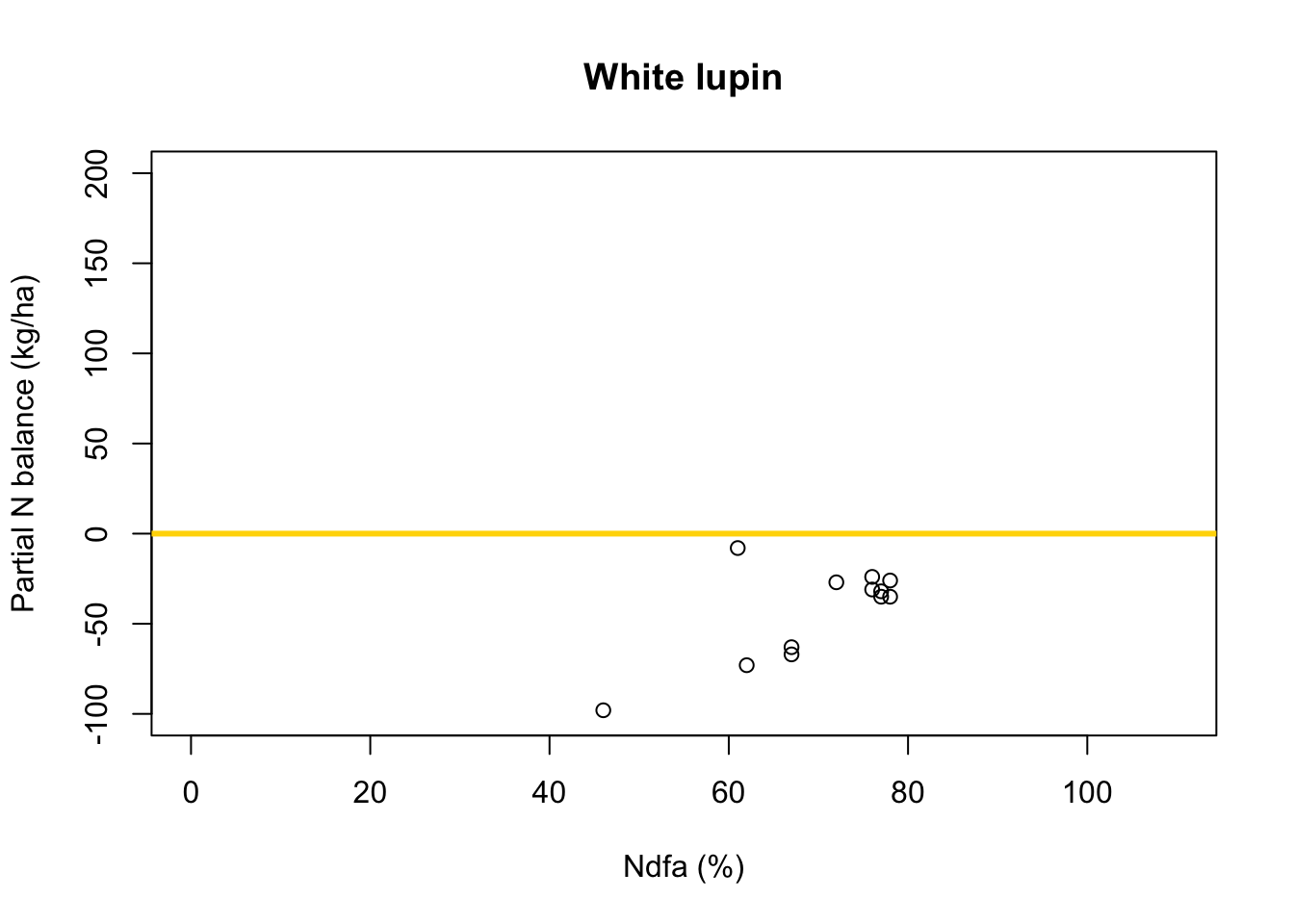
Using least squares
- What value of Ndfa is needed to achieve a neutral N balance?
beta0.hat <- as.numeric(coef(m1)[1])
beta1.hat <- as.numeric(coef(m1)[2])
theta.hat <- -beta0.hat/beta1.hat
theta.hat
## [1] 93.09456- Visual representation of \(\theta\)
# Plot data, line of best fit and theta
plot(df.wl$Ndfa,df.wl$PartNbalance,
 xlab="Ndfa (%)",ylab="Partial N balance (kg/ha)",
 xlim=c(0,110),ylim=c(-100,200),main="White lupin")
abline(a=0,b=0,col="gold",lwd=3)
abline(m1,col="red",lwd=3)
abline(v=93.1,lwd=3,lty=2,col="green")
Using likelihood-based inference
- Fit linear model to data using using maximum likelihood estimation
library(nlme) # Fit simple linear regression model using maximum likelihood estimation m2 <- gls(PartNbalance ~ Ndfa,data=df.wl,method="ML")- What value of Ndfa is needed to achieve a neutral N balance?
# Use maximum likelihood estimate (MLE) to obtain estimate of theta
beta0.hat <- as.numeric(coef(m2)[1])
beta1.hat <- as.numeric(coef(m2)[2])
theta.hat <- -beta0.hat/beta1.hat
theta.hat
## [1] 93.09456# Use delta method to obtain approximate approximate standard errors and # then construct Wald-type confidence intervals library(msm) theta.se <- deltamethod(~-x1/x2, mean=coef(m2), cov=vcov(m2)) theta.ci <- c(theta.hat-1.96*theta.se,theta.hat+1.96*theta.se) theta.ci## [1] 76.91135 109.27778- Visual representation of \(\theta\)
# Plot data, line of best fit and theta
plot(df.wl$Ndfa,df.wl$PartNbalance,
 xlab="Ndfa (%)",ylab="Partial N balance (kg/ha)",
 xlim=c(0,110),ylim=c(-100,200),main="White lupin")
abline(a=0,b=0,col="gold",lwd=3)
abline(m1,col="red",lwd=3)
abline(v=93.1,lwd=3,lty=2,col="green")
abline(v=76.9,lwd=1,lty=2,col="green")
abline(v=109.2,lwd=1,lty=2,col="green")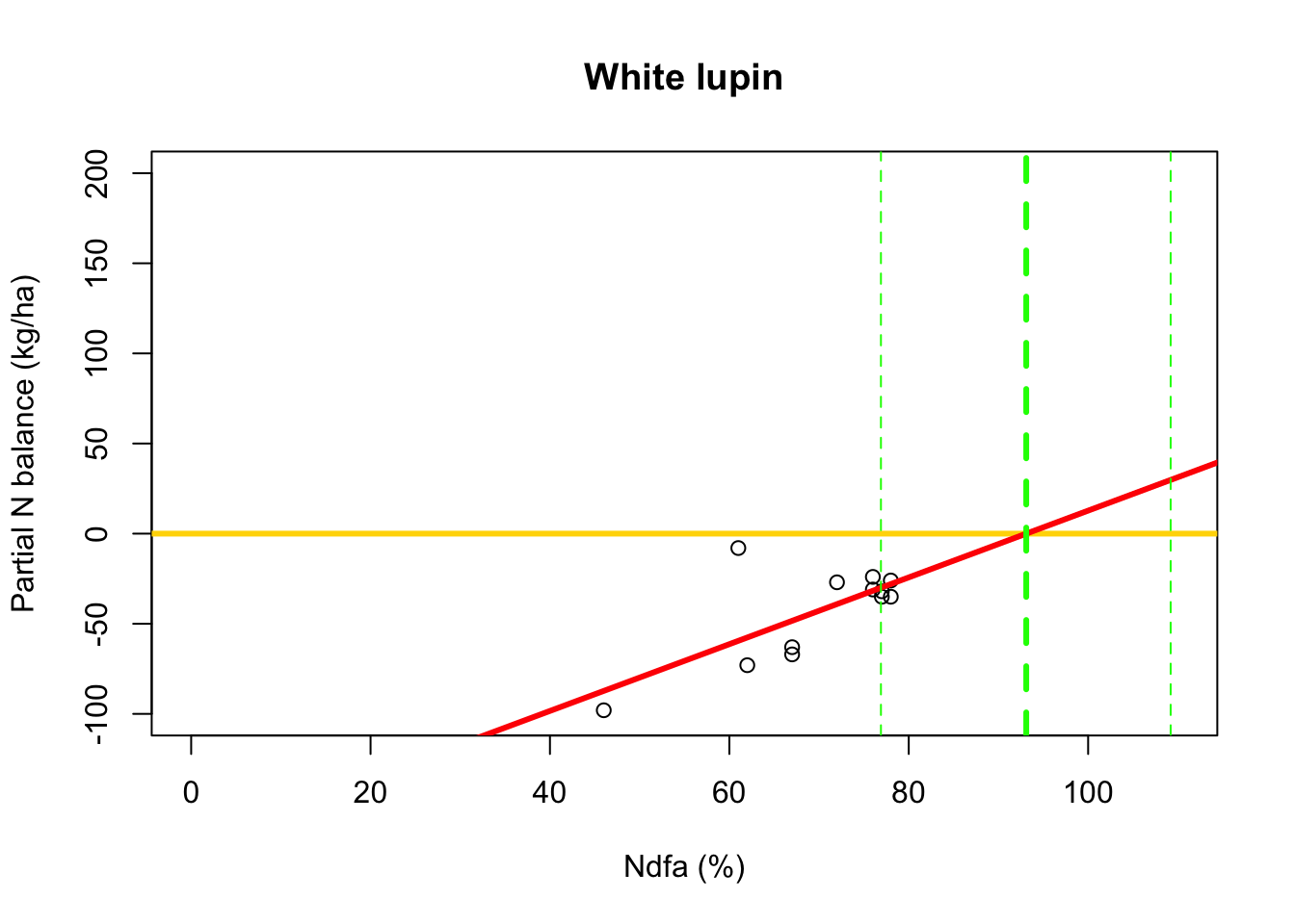
Using Bayesian inference
- Assume that \(y_i=\beta_{0}+\beta_{1}x_{i}+\varepsilon_i\) with \(\varepsilon_i\sim \text{N}(0,\sigma^2)\), \(\beta_{0}\sim \text{N}(0,10^6)\) and \(\beta_{1}\sim \text{N}(2.5,0.1)\)
- Model fitting
samples <- norm.reg.mcmc(y = df.wl$PartNbalance,X = model.matrix(~ Ndfa,data=df.wl),
                      beta.mn = c(0,2.5),beta.var=c(10^6,0.1),
                      s2.mn = 10, s2.sd = 10^6,
                      n.mcmc = 5000)

burn.in <- 1000
# Look a histograms of posterior distributions
par(mfrow=c(2,1),mar=c(5,6,1,1))
hist(samples$beta.save[1,-c(1:1000)],xlab=expression(beta[0]*"|"*bold(y)),ylab=expression("["*beta[0]*"|"*bold(y)*"]"),freq=FALSE,col="grey",main="",breaks=30)
hist(samples$beta.save[2,-c(1:1000)],xlab=expression(beta[1]*"|"*bold(y)),ylab=expression("["*beta[1]*"|"*bold(y)*"]"),freq=FALSE,col="grey",main="",breaks=30)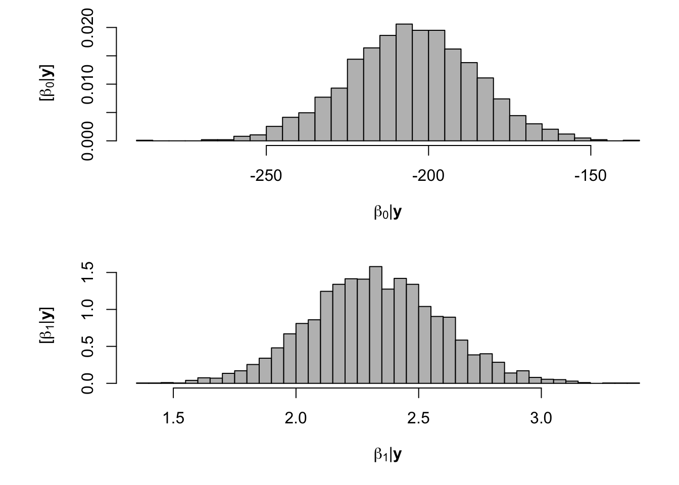
- What value of Ndfa is needed to achieve a neutral N balance?
hist(-samples$beta.save[1,-c(1:1000)]/samples$beta.save[2,-c(1:1000)],xlab=expression(theta*"|"*bold(y)),ylab=expression("["*theta*"|"*bold(y)*"]"),freq=FALSE,col="grey",main="",breaks=30)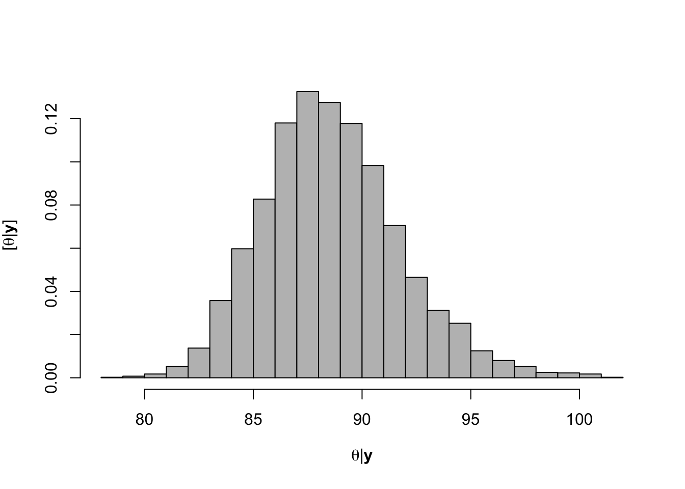
## [1] 88.59804# 95% credible intervals for theta quantile(-samples$beta.save[1,]/samples$beta.save[2,],prob=c(0.025,0.975))## 2.5% 97.5% ## 83.06360 95.69461# Plot data and theta plot(df.wl$Ndfa,df.wl$PartNbalance, xlab="Ndfa (%)",ylab="Partial N balance (kg/ha)", xlim=c(0,110),ylim=c(-100,200),main="Field pea") abline(a=0,b=0,col="gold",lwd=3) abline(v=88.6,lwd=3,lty=2,col="green") abline(v=82.7,lwd=1,lty=2,col="green") abline(v=95.7,lwd=1,lty=2,col="green") rug(-samples$beta.save[1,]/samples$beta.save[2,],col=gray(0.5,0.03))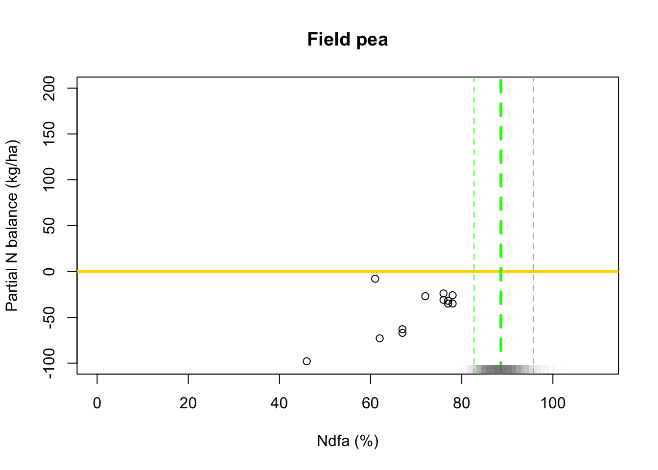
35.4 Regression trees
- Example: Change point analysis
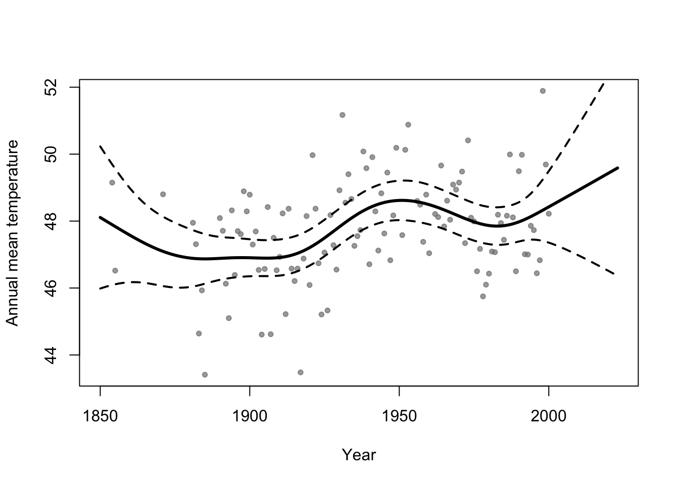
- Motivation: Annual mean temperature in Ann Arbor Michigan
library(faraway)
plot(aatemp$year,aatemp$temp,xlab="Year",ylab="Annual mean temperature",pch=20,col=rgb(0.5,0.5,0.5,0.7))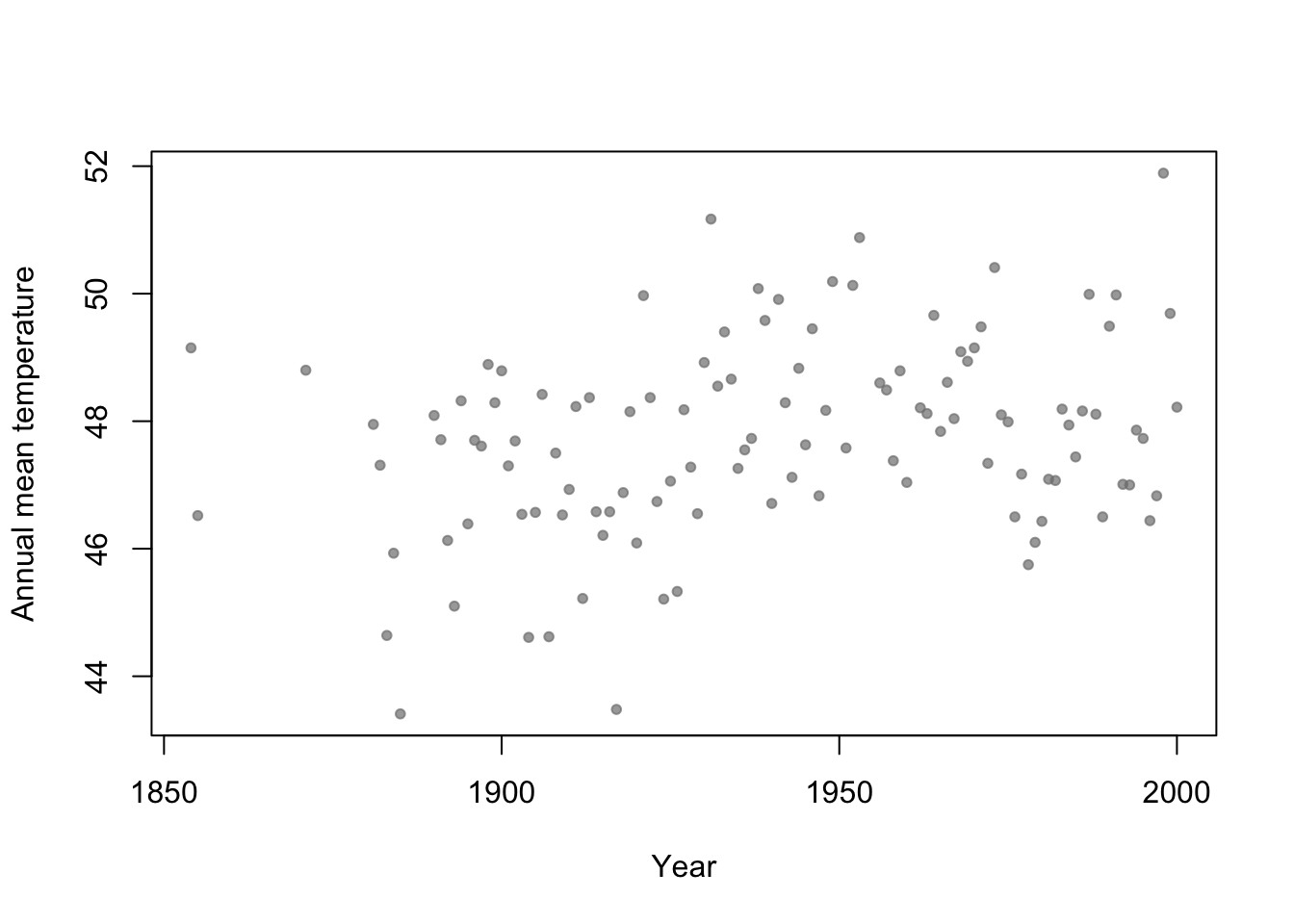
- Basis function \[f_1(x)=\begin{cases} 1 & \text{if}\;x<c\\ 0 & \text{otherwise} \end{cases}\] and \[f_2(x)=\begin{cases} 1 & \text{if}\;x\geq c\\ 0 & \text{otherwise} \end{cases}\]
- In R
# Change point basis function
f1 <- function(x,c){ifelse(x<c,1,0)}
f2 <- function(x,c){ifelse(x>=c,1,0)}

# Fit linear model
m1 <- lm(temp ~ -1 + f1(year,1930) + f2(year,1930),data=aatemp)
summary(m1)
## ## Call: ## lm(formula = temp ~ -1 + f1(year, 1930) + f2(year, 1930), data = aatemp) ## ## Residuals: ## Min 1Q Median 3Q Max ## -3.5467 -0.8962 -0.1157 1.1388 3.5843 ## ## Coefficients: ## Estimate Std. Error t value Pr(>|t|) ## f1(year, 1930) 46.9567 0.1990 236.0 <2e-16 *** ## f2(year, 1930) 48.3057 0.1684 286.8 <2e-16 *** ## --- ## Signif. codes: 0 '***' 0.001 '**' 0.01 '*' 0.05 '.' 0.1 ' ' 1 ## ## Residual standard error: 1.378 on 113 degrees of freedom ## Multiple R-squared: 0.9992, Adjusted R-squared: 0.9992 ## F-statistic: 6.899e+04 on 2 and 113 DF, p-value: < 2.2e-16# Plot predictions plot(aatemp$year,aatemp$temp,xlab="Year",ylab="Annual mean temperature",pch=20,col=rgb(0.5,0.5,0.5,0.7)) points(aatemp$year,predict(m1),type="l")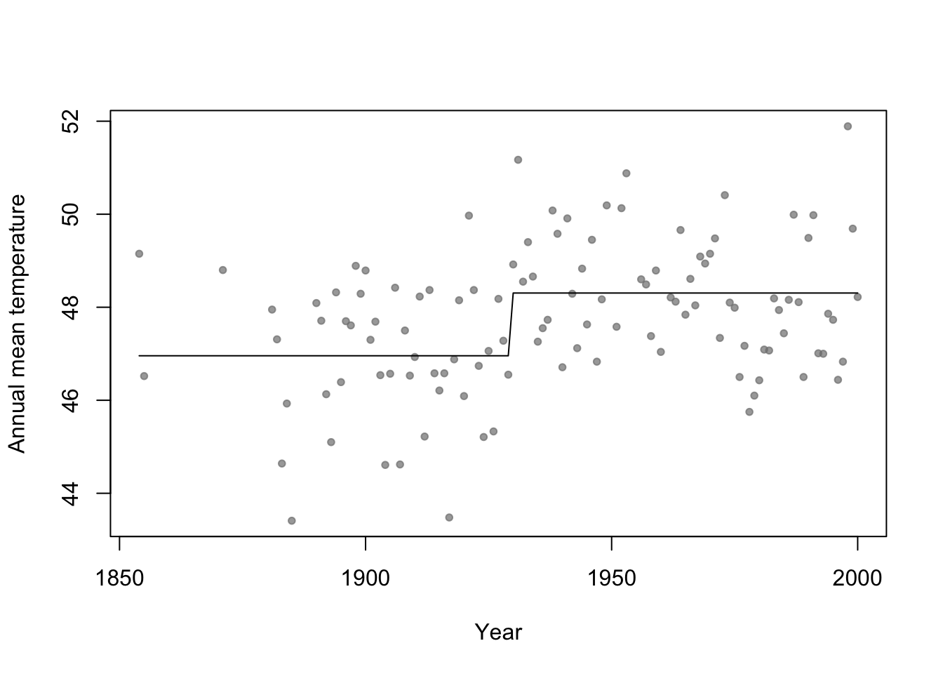
- Connection to regression trees
- For a single predictor, a regression tree can be though of as a linear model that uses the “change point” basis function, but tries to estimate the location (or time) and number of change points.
- Example in R
library(rpart)

# Fit regression tree model
m2 <- rpart(temp ~ year,data=aatemp)

# Plot predictions
E.y <- predict(m2,data.frame(year=seq(1850,2023,by=1)))
plot(aatemp$year,aatemp$temp,xlab="Year",ylab="Annual mean temperature",pch=20,col=rgb(0.5,0.5,0.5,0.7),xlim=c(1850,2023))
points(1850:2023,E.y,type="l")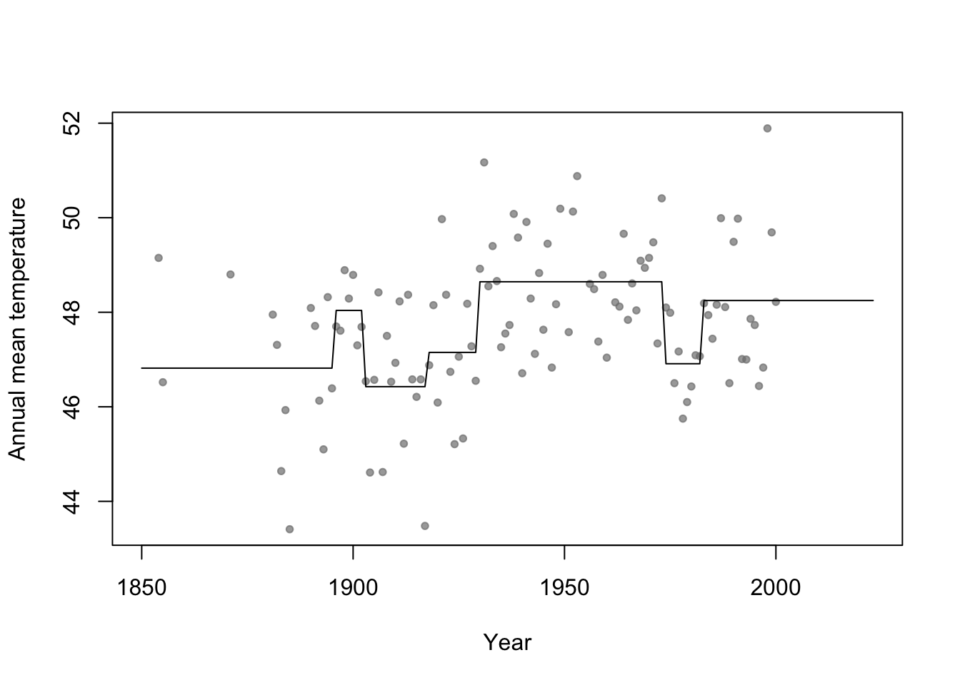
35.5 Random forest
Breiman 2001 link
Example
n.boot <- 1000 # Number of bootstrap samples
x.new=seq(1850,2023,by=1) # New values of x that I want predicitons at
E.y <- matrix(,length(x.new),n.boot) # Matrix to save predictions
x <- aatemp$year
y <- aatemp$temp

for(i in 1:n.boot){

  # Resample data
  df.temp <- data.frame(y=y,x=x)[sample(1:length(y),replace=TRUE,size=51),]

  # Fit tree
  m1 <- rpart(y~x,data=df.temp)

  # Get and save predictions
  E.y[,i] <- predict(m1,data.frame(x=x.new))
}

plot(aatemp$year,aatemp$temp,xlab="Year",ylab="Annual mean temperature",pch=20,col=rgb(0.5,0.5,0.5,0.7),xlim=c(1850,2023))


# Aggregate predictions
E.E.y <- rowMeans(E.y)
points(1850:2023,E.E.y,type="l")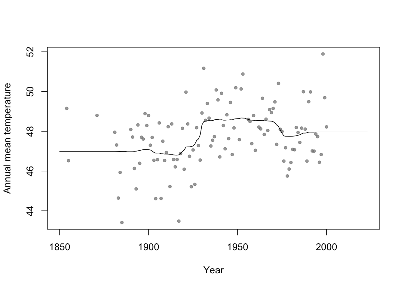
Summary
- Bootstrap aggregating (or bagging) can be used with any statistical model
- Usually increases predictive accuracy but reduces ability to understand (and write-out) the model(s) and make inference
35.6 Generalized additive model
Write out on white board
Difference between interpretable vs. non-interpretable model/machine learning approaches
My personal use of gams
- The functions lm() and glm() and packages lme4, nlme, etc
- Why I use the mgcv package
- Wood (2017)
- The functions lm() and glm() and packages lme4, nlme, etc
Example
library(faraway)
library(mgcv)

m1 <- gam(temp ~ s(year,bs="tp"),family=Gamma(link="log"),data=aatemp)

# Plot predictions
E.y <- predict(m1,data.frame(year=seq(1850,2023,by=1)),type="response")
ui <- E.y + 1.96*predict(m1,data.frame(year=seq(1850,2023,by=1)),type="response",se=TRUE)$se.fit
li <- E.y - 1.96*predict(m1,data.frame(year=seq(1850,2023,by=1)),type="response",se=TRUE)$se.fit
plot(aatemp$year,aatemp$temp,xlab="Year",ylab="Annual mean temperature",pch=20,col=rgb(0.5,0.5,0.5,0.7),xlim=c(1850,2023))
points(1850:2023,E.y,type="l",lwd=3)
points(1850:2023,ui,type="l",lwd=2,lty=2)
points(1850:2023,li,type="l",lwd=2,lty=2)