32 Day 31 (July 19)
32.1 Announcements
Please email me and request a 20 min time period during the final week of class (July 22 - 26) to give your final presentation. When you email me please suggest three times/dates that work for you.
Read Ch. 10 in linear models with R
Up next
- Random effects/mixed model
- Generalized linear models
- Machine learning (e.g., regression trees, random forest)
32.2 Model selection
- Recall that all inference is conditional on the statistical model that we have chosen to use.
- Components of a statistical model
- Are the assumptions met?
- Are there better models we could have used?
- What should you do if you have two or more competing models?
- Information criterion
- Motivation: Adjusted \(R^2\)
- Recall \[\hat{R}^{2}=1-\frac{(\mathbf{y}-\mathbf{X}\hat{\boldsymbol{\beta}})^{\prime}(\mathbf{y}-\mathbf{X}\hat{\boldsymbol{\beta})}}{(\mathbf{y}-\mathbf{1}\hat{\beta}_{0})^{\prime}(\mathbf{y}-\mathbf{1}\hat{\beta}_{0})}\]
- As we add more predictors to \(\mathbf{X}\), \(R^{2}\) monotonically increases when calculated using in-sample data.
- Calculating \(R^{2}\) using in-sample data results in a biased estimator of the \(R^{2}\) calculated using “out-of-sample” (i.e., \(\text{E}(\hat{R}_{\text{in-sample}}^{2})\neq R_{\text{out-of-sample}}^{2}\))
- Adjusted \(R^{2}\) is a biased corrected version of \(R^{2}\). \[\hat{R}^{2}_{\text{adjusted}}=1-\bigg{(}\frac{n-1}{n-p}\bigg{)}\frac{(\mathbf{y}-\mathbf{X}\hat{\boldsymbol{\beta}})^{\prime}(\mathbf{y}-\mathbf{X}\hat{\boldsymbol{\beta})}}{(\mathbf{y}-\mathbf{1}\hat{\beta}_{0})^{\prime}(\mathbf{y}-\mathbf{1}\hat{\beta}_{0})}\]
- Many different estimators exist for adjusted \(R^{2}\)
- Different assumptions lead to different estimators
- Gelman, Hwang, and Vehtari (2014) on estimating out-of-sample predictive accuracy using in-sample data
- “We know of no approximation that works in general….Each of these methods has flaws, which tells us that any predictive accuracy measure that we compute will be only approximate”
- “One difficulty is that all the proposed measures are attempting to perform what is, in general, an impossible task: to obtain an unbiased (or approximately unbiased) and accurate measure of out-of-sample prediction error that will be valid over a general class of models…”
- Motivation: Adjusted \(R^2\)
- Akaike’s Information Criterion
- The log-likelihood as a scoring rule \[\mathcal{l}(\boldsymbol{\theta}|\mathbf{y})\]
- The log-likelihood for the linear model \[\mathcal{l}(\boldsymbol{\beta},\sigma^2|\mathbf{y})=-\frac{n}{2}\text{ log}(2\pi\sigma^2) - \frac{1}{2\sigma^2}\sum_{i=1}^{n}(y_{i} - \mathbf{x}_{i}^{\prime}\boldsymbol{\beta})^2.\]
- Like \(R^2\), \(\mathcal{l}(\boldsymbol{\beta},\sigma^2|\mathbf{y})\) can be used to measure predictive accuracy on in-sample or out of sample data.
- Unlike \(R^2\), the log-likelihood is a general scoring rule. For example, let \(\mathbf{y} \sim \text{Bernoulli}(p)\) then \[\sum_{i=1}^{n}y_{i}\text{log}(p)+(1-y_{i})\text{log}({1-p}).\]
- The log-likelihood is a relative score and can be difficult to interpret.
- AIC uses the in-sample log-likelihood, but achieves an (asymptotically) unbiased estimate the log-likelihood on the out-of-sample data by adding a bias correction. The statistic is then multiplied by negative two \[AIC=-2\mathcal{l}(\boldsymbol{\theta}|\mathbf{y}) + 2q\]
- What is a meaninful difference in AIC?
- AIC is a derived quanitity. Just like \(R^2\) we can and should get measures of uncertainty (e.g., 95% CI).
- Example
- Motivation: Annual mean temperature in Ann Arbor Michigan
library(faraway)
plot(aatemp$year,aatemp$temp,xlab="Year",ylab="Annual mean temperature",pch=20,col=rgb(0.5,0.5,0.5,0.7))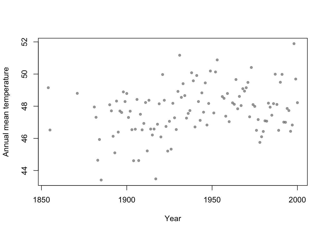
df.in_sample <- aatemp # Use all years for in-sample data

# Intercept only model
m1 <- lm(temp ~ 1,data=df.in_sample)

# Simple regression model
m2 <- lm(temp ~ year,data=df.in_sample)

par(mfrow=c(1,1))
# Plot predictions (in-sample)
plot(df.in_sample$year,df.in_sample$temp,main="In-sample",xlab="Year",ylab="Annual mean temperature",ylim=c(44,52),pch=20,col=rgb(0.5,0.5,0.5,0.7))
lines(df.in_sample$year,predict(m2))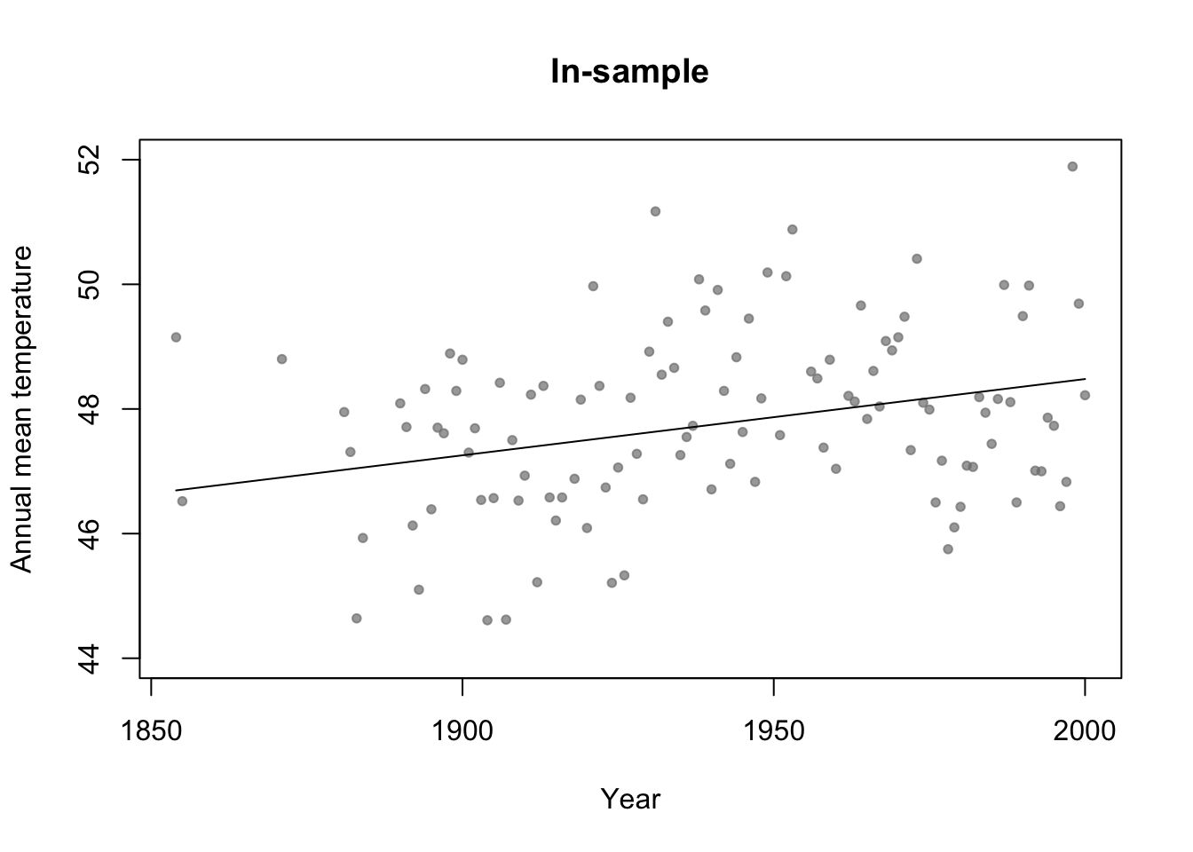
# Broken stick basis function
f1 <- function(x,c){ifelse(x<c,c-x,0)}
f2 <- function(x,c){ifelse(x>=c,x-c,0)}
m3 <- lm(temp ~ f1(year,1930) + f2(year,1930),data=df.in_sample)

par(mfrow=c(1,1))
# Plot predictions (in-sample)
plot(df.in_sample$year,df.in_sample$temp,main="In-sample",xlab="Year",ylab="Annual mean temperature",ylim=c(44,52),pch=20,col=rgb(0.5,0.5,0.5,0.7))
lines(df.in_sample$year,predict(m3))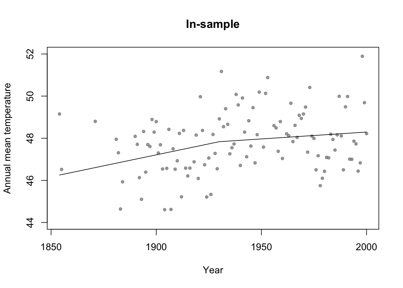
library(rpart)
# Fit regression tree model
m4 <- rpart(temp ~ year,data=df.in_sample)

par(mfrow=c(1,1))
# Plot predictions (in-sample)
plot(df.in_sample$year,df.in_sample$temp,main="In-sample",xlab="Year",ylab="Annual mean temperature",ylim=c(44,52),pch=20,col=rgb(0.5,0.5,0.5,0.7))
lines(df.in_sample$year,predict(m4))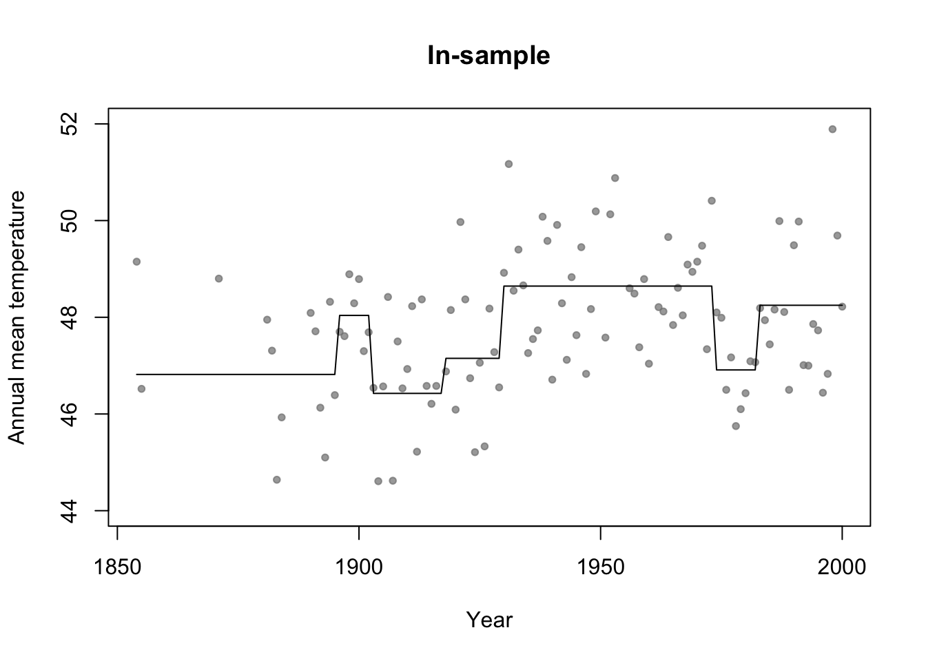
## [1] 0## [1] 0.0772653## [1] 0.07692598# Not clear how to calculate adjusted R^2 for m4 (regression tree)
# AIC
y <- df.in_sample$temp
y.hat_m1 <- predict(m1,newdata=df.in_sample)
y.hat_m2 <- predict(m2,newdata=df.in_sample)
y.hat_m3 <- predict(m3,newdata=df.in_sample)
y.hat_m4 <- predict(m4,newdata=df.in_sample)
sigma2.hat_m1 <- summary(m1)$sigma^2
sigma2.hat_m2 <- summary(m2)$sigma^2
sigma2.hat_m3 <- summary(m3)$sigma^2
# m1
#log-likelihood
ll <- sum(dnorm(y,y.hat_m1,sigma2.hat_m1^0.5,log=TRUE)) # same as logLik(m1)
q <- 1 + 1 # number of estimated betas + number estimated sigma2s
#AIC
-2*ll+2*q #Same as AIC(m1)## [1] 426.6276# m2
#log-likelihood
ll <- sum(dnorm(y,y.hat_m2,sigma2.hat_m2^0.5,log=TRUE)) # same as logLik(m2)
q <- 2 + 1 # number of estimated betas + number estimated sigma2s
#AIC
-2*ll+2*q #Same as AIC(m2)## [1] 418.38# m3
#log-likelihood
ll <- sum(dnorm(y,y.hat_m3,sigma2.hat_m3^0.5,log=TRUE)) # same as logLik(m3)
q <- 3 + 1 # number of estimated betas + number estimated sigma2s
#AIC
-2*ll+2*q #Same as AIC(m3)## [1] 419.4223# m4
n <- length(y)
q <- 7 + 6 + 1 # number of estimated "intercept" terms in each termimal node + number of estimated "breaks" + number estimated sigma2s
sigma2.hat_m4 <- t(y - y.hat_m4)%*%(y - y.hat_m4)/(n - q - 1)
# log-likelihood
ll <- sum(dnorm(y,y.hat_m4,sigma2.hat_m4^0.5,log=TRUE))
#AIC
-2*ll+2*q## [1] 406.5715Example: assessing uncertainity in model selection statistics
library(mosaic)

boot <- function(){
m1 <- lm(temp ~ 1,data=resample(df.in_sample))
m2 <- lm(temp ~ year,data=resample(df.in_sample))
m3 <- lm(temp ~ f1(year,1930) + f2(year,1930),data=resample(df.in_sample))
cbind(AIC(m1),AIC(m2),AIC(m3))}

bs.aic.samplles <- do(1000)*boot()

par(mfrow=c(3,1))
hist(bs.aic.samplles[,1],col="grey",main="m1",freq=FALSE,xlab="AIC score",xlim=range(bs.aic.samplles))
abline(v=AIC(m1),col="gold",lwd=3)
hist(bs.aic.samplles[,2],col="grey",main="m2",freq=FALSE,xlab="AIC score",xlim=range(bs.aic.samplles))
abline(v=AIC(m2),col="gold",lwd=2)
hist(bs.aic.samplles[,3],col="grey",main="m3",freq=FALSE,xlab="AIC score",xlim=range(bs.aic.samplles))
abline(v=AIC(m3),col="gold",lwd=3)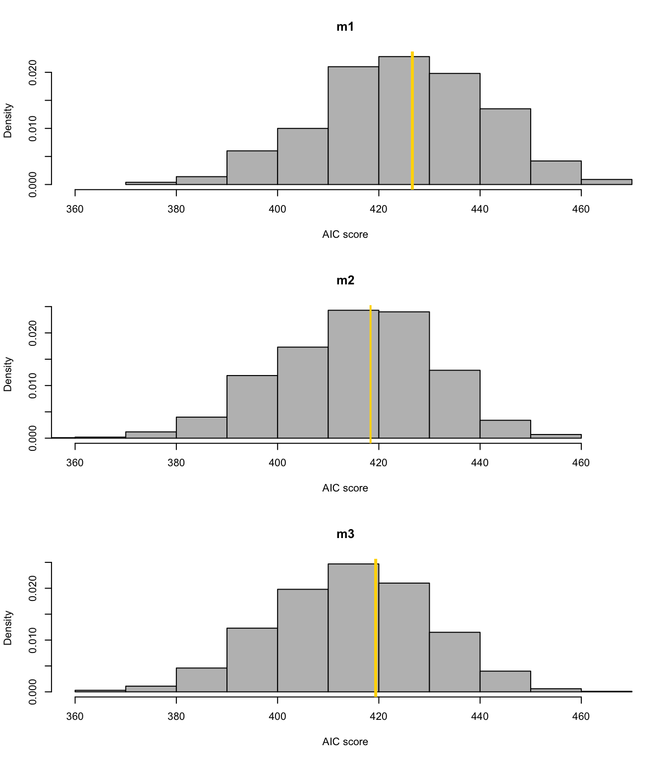
Summary
- Making statistical inference after model selection?
- Discipline specific views (e.g., AIC in wildlife ecology).
- There are many choices for model selection using in-sample data. Knowing the “best” model selection approach would require you to know a lot about all other procedures.
- AIC (Akaike 1973)
- BIC (Swartz 1978)
- CAIC (Vaida & Blanchard 2005)
- DIC (Spiegelhalter et al. 2002)
- ERIC (Hui et al. 2015)
- And the list goes on
- I would recommend using methods that you understand.
- In my experience it takes a larger data set to do estimation and model selection
- If you have a large data set, split it and use out-of-sample data for estimation
- If you don’t have a large data set, make sure you assess the uncertainty. You might not have enough data to do both estimation and model selection.
32.3 Random effects
Conditional, marginal, and joint distributions
- Conditional distribution: “\(\mathbf{y}\) given \(\boldsymbol{\beta}\)” \[\mathbf{y}|\boldsymbol{\beta}\sim\text{N}(\mathbf{X}\boldsymbol{\beta},\sigma_{\varepsilon}^{2}\mathbf{I})\] This is also sometimes called the data model.
- Marginal distribution of \(\boldsymbol{\beta}\) \[\beta\sim\text{N}(\mathbf{0},\sigma_{\beta}^{2}\mathbf{I})\] This is also called the parameter model.
- Joint distribution \([\mathbf{y}|\boldsymbol{\beta}][\boldsymbol{\beta}]\)
Estimation for the linear model with random effects
- By maximizing the joint likelihood
- Write out the likelihood function \[\mathcal{L}(\boldsymbol{\beta},\sigma_{\varepsilon},\sigma_{\beta}^{2})=\frac{1}{(2\pi)^{-\frac{n}{2}}}|\sigma^{2}_{\varepsilon}\mathbf{I}|^{-\frac{1}{2}}\text{exp}\bigg{(}-\frac{1}{2}(\mathbf{y} - \mathbf{X}\boldsymbol{\beta})^{\prime}(\sigma^{2}_{\varepsilon}\mathbf{I})^{-1}(\mathbf{y} - \mathbf{X}\boldsymbol{\beta})\bigg{)}\times\\\frac{1}{(2\pi)^{-\frac{p}{2}}}|\sigma^{2}_{\beta}\mathbf{I}|^{-\frac{1}{2}}\text{exp}\bigg{(}-\frac{1}{2}\boldsymbol{\beta}^{\prime}(\sigma^{2}_{\beta}\mathbf{I})^{-1}\boldsymbol{\beta}\bigg{)}\]
- Maximizing the log-likelihood function w.r.t. gives \(\boldsymbol{\beta}\) gives \[\hat{\boldsymbol{\beta}}=\big{(}\mathbf{X}^{'}\mathbf{X}+\frac{\sigma^{2}_{\varepsilon}}{\sigma^{2}_{\beta}}\mathbf{I}\big{)}^{-1}\mathbf{X}^{'}\mathbf{y}\]
- By maximizing the joint likelihood
Example eye temperature data set for Eurasian blue tit
df.et <- read.table("https://www.dropbox.com/s/bo11n66cezdnbia/eyetemp.txt?dl=1")
names(df.et) <- c("id","sex","date","time","event","airtemp","relhum","sun","bodycond","eyetemp")
df.et$id <- as.factor(df.et$id)
df.et$id.num <- as.numeric(df.et$id)

ind.means <- aggregate(eyetemp ~ id.num,df.et, FUN=base::mean)
plot(df.et$id.num,df.et$eyetemp,xlab="Individual",ylab="Eye temperature")
points(ind.means,pch="x",col="gold",cex=1.5)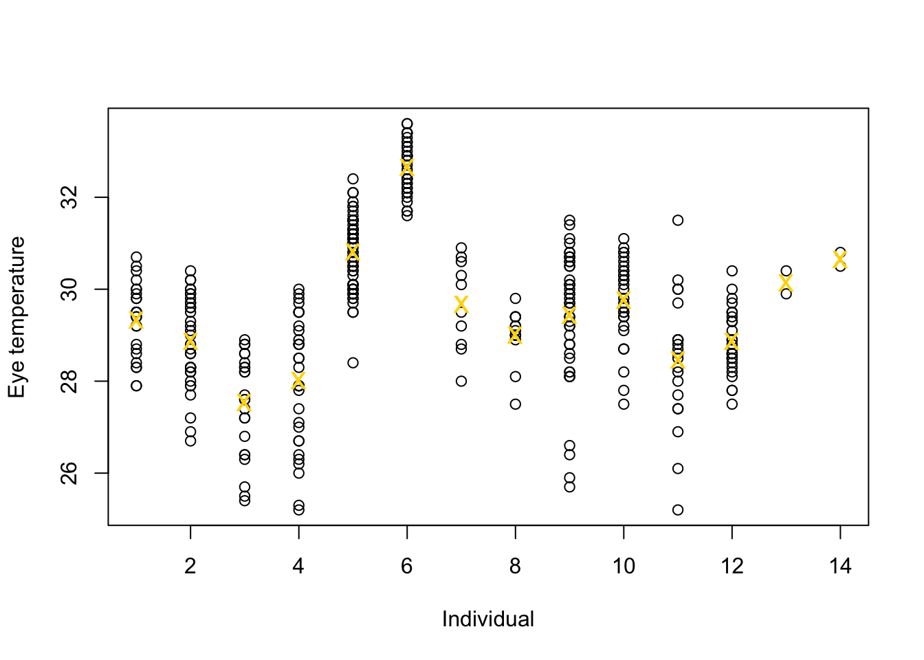
# Standard "fixed effects" linear regression model
m1 <- lm(eyetemp~as.factor(id.num)-1,data=df.et)
summary(m1)
## ## Call: ## lm(formula = eyetemp ~ as.factor(id.num) - 1, data = df.et) ## ## Residuals: ## Min 1Q Median 3Q Max ## -3.7378 -0.5750 0.1507 0.6622 3.0286 ## ## Coefficients: ## Estimate Std. Error t value Pr(>|t|) ## as.factor(id.num)1 29.3423 0.1972 148.77 <2e-16 *** ## as.factor(id.num)2 28.8735 0.1725 167.41 <2e-16 *** ## as.factor(id.num)3 27.5458 0.2053 134.19 <2e-16 *** ## as.factor(id.num)4 28.0156 0.1778 157.59 <2e-16 *** ## as.factor(id.num)5 30.8188 0.1211 254.56 <2e-16 *** ## as.factor(id.num)6 32.6486 0.1700 192.06 <2e-16 *** ## as.factor(id.num)7 29.6800 0.3180 93.33 <2e-16 *** ## as.factor(id.num)8 29.0000 0.2789 103.97 <2e-16 *** ## as.factor(id.num)9 29.4378 0.1499 196.36 <2e-16 *** ## as.factor(id.num)10 29.7667 0.1836 162.12 <2e-16 *** ## as.factor(id.num)11 28.4714 0.2195 129.74 <2e-16 *** ## as.factor(id.num)12 28.8793 0.1867 154.64 <2e-16 *** ## as.factor(id.num)13 30.1500 0.7111 42.40 <2e-16 *** ## as.factor(id.num)14 30.6500 0.7111 43.10 <2e-16 *** ## --- ## Signif. codes: 0 '***' 0.001 '**' 0.01 '*' 0.05 '.' 0.1 ' ' 1 ## ## Residual standard error: 1.006 on 358 degrees of freedom ## Multiple R-squared: 0.9989, Adjusted R-squared: 0.9989 ## F-statistic: 2.31e+04 on 14 and 358 DF, p-value: < 2.2e-16plot(df.et$id.num,df.et$eyetemp,xlab="Individual",ylab="Expected eye temperature",col="white") points(1:14,coef(m1),pch=20,col="black",cex=1) segments (1:14,confint(m1)[,1],1:14,confint(m1)[,2] ,lwd=2,lty=1)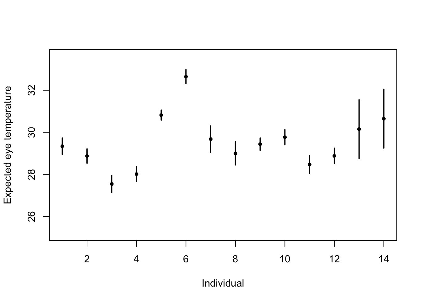
# Random effects regression model (using nlme package; difficult to get confidence interval)
library(nlme)
m2 <- lme(fixed = eyetemp ~ 1,random= list(id = pdIdent(~id-1)),data=df.et,method="ML")#summary(m2)
#predict(m2,level=1,newdata=data.frame(id=unique(df.et$id)))

# Random effects regression model (mgcv package)
library(mgcv)
m2 <- gam(eyetemp ~ 1+s(id,bs="re"),data=df.et,method="ML")

plot(df.et$id.num,df.et$eyetemp,xlab="Individual",ylab="Expected eye temperature",col="white")
points(1:14-0.15,coef(m1),pch=20,col="black",cex=1)
segments (1:14-0.15,confint(m1)[,1],1:14-0.15,confint(m1)[,2] ,lwd=2,lty=1)
pred <- predict(m2,newdata=data.frame(id=unique(df.et$id)),se.fit=TRUE)
pred$lci <- pred$fit - 1.96*pred$se.fit
pred$uci <- pred$fit + 1.96*pred$se.fit
points(1:14+0.15,pred$fit,pch=20,col="green",cex=1)
segments (1:14+0.15,pred$lci,1:14+0.15,pred$uci,lwd=2,lty=1,col="green")
abline(a=coef(m2)[1],b=0,col="grey")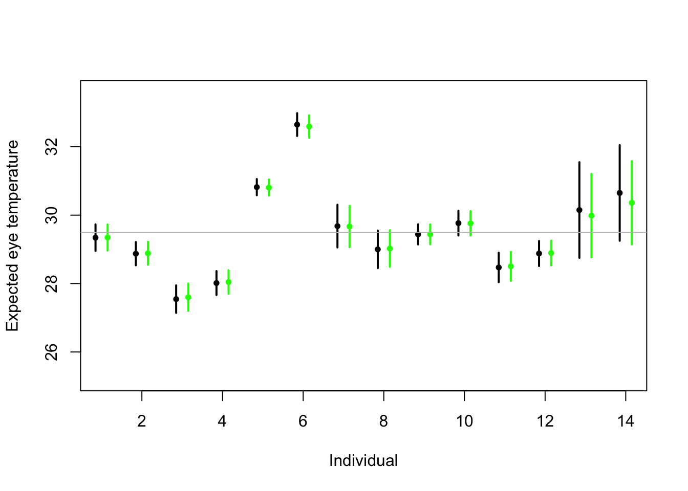
Summary
- Take home message
- Treating \(\boldsymbol{\beta}\) as a random effect “shrinks” the estimates of \(\boldsymbol{\beta}\) closer to zero.
- Requires an extra assumption \(\boldsymbol{\beta}\sim\text{N}(\mathbf{0},\sigma_{\beta}^{2}\mathbf{I})\)
- Penalty
- Random effect
- This called a prior distribution in Bayesian statistics
- Take home message
32.4 Generalized linear models
The generalized linear model framework \[\mathbf{y} \sim[\mathbf{\mathbf{y}|\boldsymbol{\mu},\psi]}\] \[g(\boldsymbol{\mu})=\mathbf{X}\boldsymbol{\beta}\]
- \([\mathbf{y}|\boldsymbol{\mu},\psi]\) is a distribution from the exponential family (e.g., normal, Poisson, binomial) with expected value \(\boldsymbol{\mu}\) and dispersion parameter \(\psi\).
- Example \([\mathbf{y}|\boldsymbol{\mu},\psi]=\text{N}\left(\boldsymbol{\mu},\psi\mathbf{I}\right)\)
- Example \([\mathbf{\mathbf{y}|\boldsymbol{\mu},\psi]}=\text{Poisson}\left(\boldsymbol{\mu}\right)\)
- Example \([\mathbf{\mathbf{y}|\boldsymbol{\mu},\psi]}=\text{gamma}\left(\boldsymbol{\mu},\psi\right)\)
- \([\mathbf{y}|\boldsymbol{\mu},\psi]\) is a distribution from the exponential family (e.g., normal, Poisson, binomial) with expected value \(\boldsymbol{\mu}\) and dispersion parameter \(\psi\).
Estimation
- Use numerical maximization to estimate
- \(\hat{\boldsymbol{\beta}}=(\mathbf{X}^{\prime}\mathbf{X})^{-1}\mathbf{X}^{\prime}\mathbf{y}\) is NOT the MLE for the glm
- Inference is based on asymptotic properties of MLE.
- Example: Challenger data
- The statistical model: \[\mathbf{y}\sim\text{binomial}(6,\mathbf{p})\] \[\text{logit}(\mathbf{p})=\mathbf{X}\boldsymbol{\beta}.\]
- The PMF for the binomial distribution \[\binom{N}{y}p^{y}(1-p)^{N-y}\]
- Write out the likelihood function \[\mathcal{L}(\boldsymbol{\beta})=\prod_{i=1}^n\binom{6}{y_i}p_i^{y_i}(1-p_i)^{6-y_i}\]
- Maximize the log-likelihood function
challenger <- read.csv("https://www.dropbox.com/s/ezxj8d48uh7lzhr/challenger.csv?dl=1")

plot(challenger$Temp,challenger$O.ring,xlab="Temperature",ylab="Number of incidents",xlim=c(10,80),ylim=c(0,6))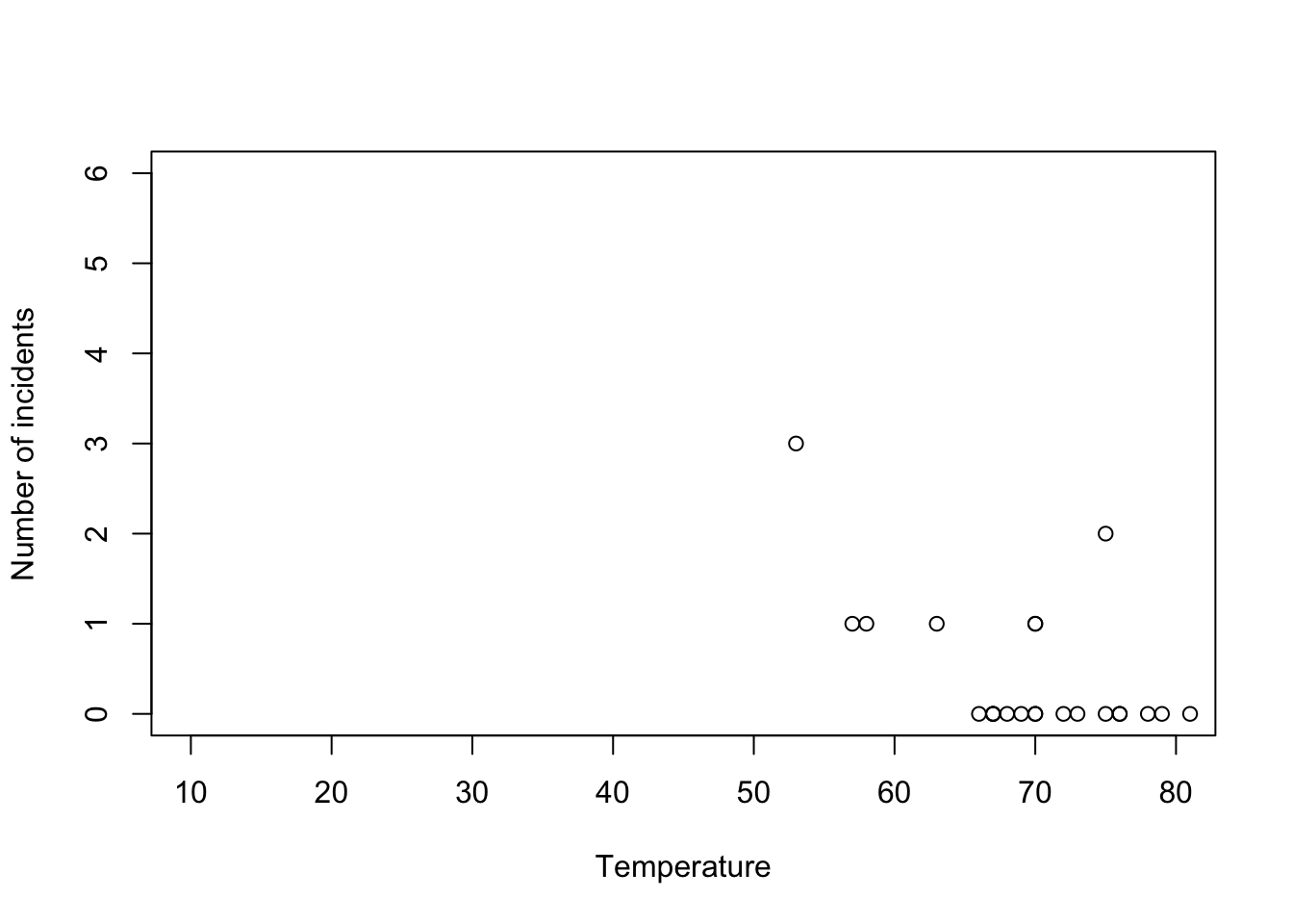
y <- challenger$O.ring
X <- model.matrix(~Temp,data= challenger)

nll <- function(beta){
  p <- 1/(1+exp(-X%*%beta)) # Inverse of logit link function
  -sum(dbinom(y,6,p,log=TRUE)) # Sum of the log likelihood for each observation
  }
est <- optim(par=c(0,0),fn=nll,hessian=TRUE)

# MLE of beta
est$par
## [1] 6.751192 -0.139703## [1] 8.830866682 0.002145791## [1] 2.97167742 0.04632268- Using the
glm()function
m1 <- glm(cbind(challenger$O.ring,6-challenger$O.ring) ~ Temp, family = binomial(link = "logit"),data=challenger)
summary(m1)
## ## Call: ## glm(formula = cbind(challenger$O.ring, 6 - challenger$O.ring) ~ ## Temp, family = binomial(link = "logit"), data = challenger) ## ## Coefficients: ## Estimate Std. Error z value Pr(>|z|) ## (Intercept) 6.75183 2.97989 2.266 0.02346 * ## Temp -0.13971 0.04647 -3.007 0.00264 ** ## --- ## Signif. codes: 0 '***' 0.001 '**' 0.01 '*' 0.05 '.' 0.1 ' ' 1 ## ## (Dispersion parameter for binomial family taken to be 1) ## ## Null deviance: 28.761 on 22 degrees of freedom ## Residual deviance: 19.093 on 21 degrees of freedom ## AIC: 36.757 ## ## Number of Fisher Scoring iterations: 5- Prediction
- We can get prediction using \(\mathbf{X}\hat{\boldsymbol{\beta}}\) or the inverse of the logit link function \(\hat{\boldsymbol{\mu}}=\frac{1}{1+e^{-\mathbf{X}\hat{\boldsymbol{\beta}}}}\)
- Confidence intervals for \(\mathbf{X}\hat{\boldsymbol{\beta}}\) are straightforward
- Confidence intervals for \(\hat{\boldsymbol{\mu}}=\frac{1}{1+e^{-\mathbf{X}\hat{\boldsymbol{\beta}}}}\) are not straightforward because of the nonlinear transformation of \(\hat{\boldsymbol{\beta}}\)
beta.hat <- coef(m1)

new.temp <- seq(0,80,by=0.01)
X.new <- model.matrix(~new.temp)

mu.hat <- (1/(1+exp(-X.new%*%beta.hat)))

plot(challenger$Temp,challenger$O.ring,xlab="Temperature",ylab="Number of incidents",xlim=c(10,80),ylim=c(0,6))
points(new.temp,6*mu.hat,typ="l",col="red")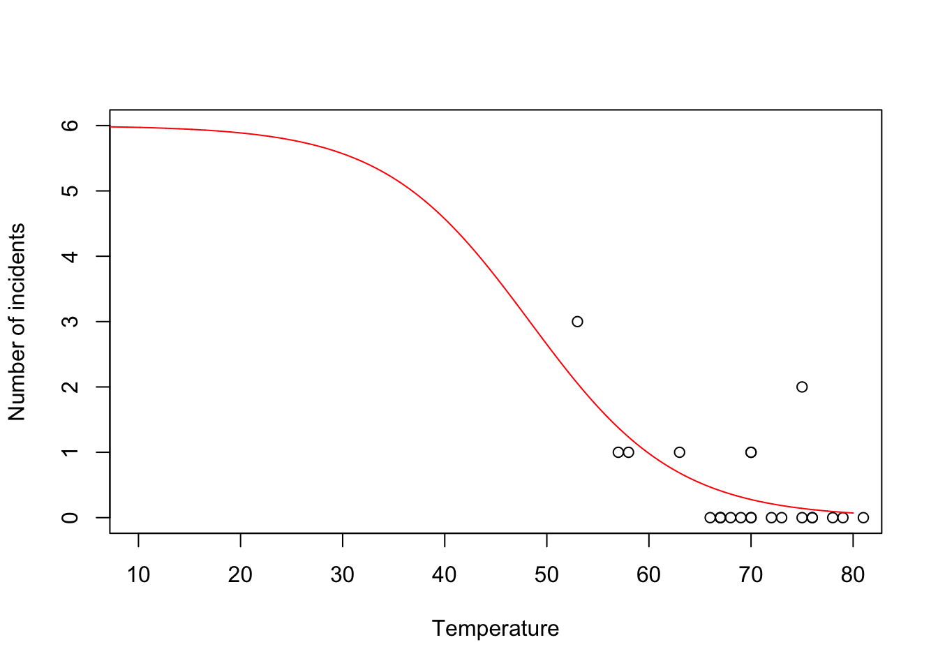
- Predictive distribution
library(mosaic)

predict.bs <- function(){
  m1 <- glm(cbind(O.ring,6-O.ring) ~ Temp, family = binomial(link = "logit"),data=resample(challenger))
  p <- predict(m1,newdata=data.frame(Temp=31),type="response")
  y <- rbinom(1,6,p)
  y
}

bootstrap <- do(1000)*predict.bs()

par(mar = c(5, 4, 7, 2))
hist(bootstrap[,1], col = "grey", xlab = "Year", main = "Empirical distribution of O-ring failures at 31 degrees", freq = FALSE,right=FALSE,breaks=c(-0.5:6.5))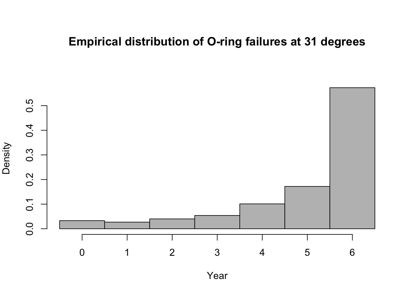
# 95% equal-tailed CI based on percentiles of the empirical distribution
quantile(bootstrap[,1], prob = c(0.025, 0.975))
## 2.5% 97.5% ## 0 6## [1] 0.573Summary
- The generalized linear model useful when the distributional assumptions of linear model are untenable.
- Small counts
- Binary data
- Two cultures
- All distributions are approximations of a unknown data generating process so why does it matter? Use the linear model because it is easier to understand.
- Personal philosophy
- Picking a distribution whose support matches that of the data gets closer to the etiology of the process that generated the data.
- Easier for me to think scientifically about the process
- The generalized linear model useful when the distributional assumptions of linear model are untenable.
32.5 Transformations of the response
Big picture idea
- Select a function that transforms \(\mathbf{y}\) such that the assumptions of normality are approximately correct.
Two cultures
- This is with respect to \(\mathbf{y}\) and not the predictors. Transforming the predictors is not at all controversial.
- Trade offs
- Difficult to apply sometimes (e.g., \(\text{log(}\mathbf{y}+c)\) for count data)
- Difficult to interpret on the transformed scale
- If normality is an appropriate assumption, we can use the general linear model \(\textbf{y}\sim\text{N}(\mathbf{X}\boldsymbol{\beta},\mathbf{V})\)
Example
- Number of whooping cranes each year
url <- "https://www.dropbox.com/s/ihs3as87oaxvmhq/Butler%20et%20al.%20Table%201.csv?dl=1"
df1 <- read.csv(url)
plot(df1$Winter,df1$N,typ="b",xlab="Year",ylab="Population Size",ylim=c(0,300),lwd=1.5,pch="*")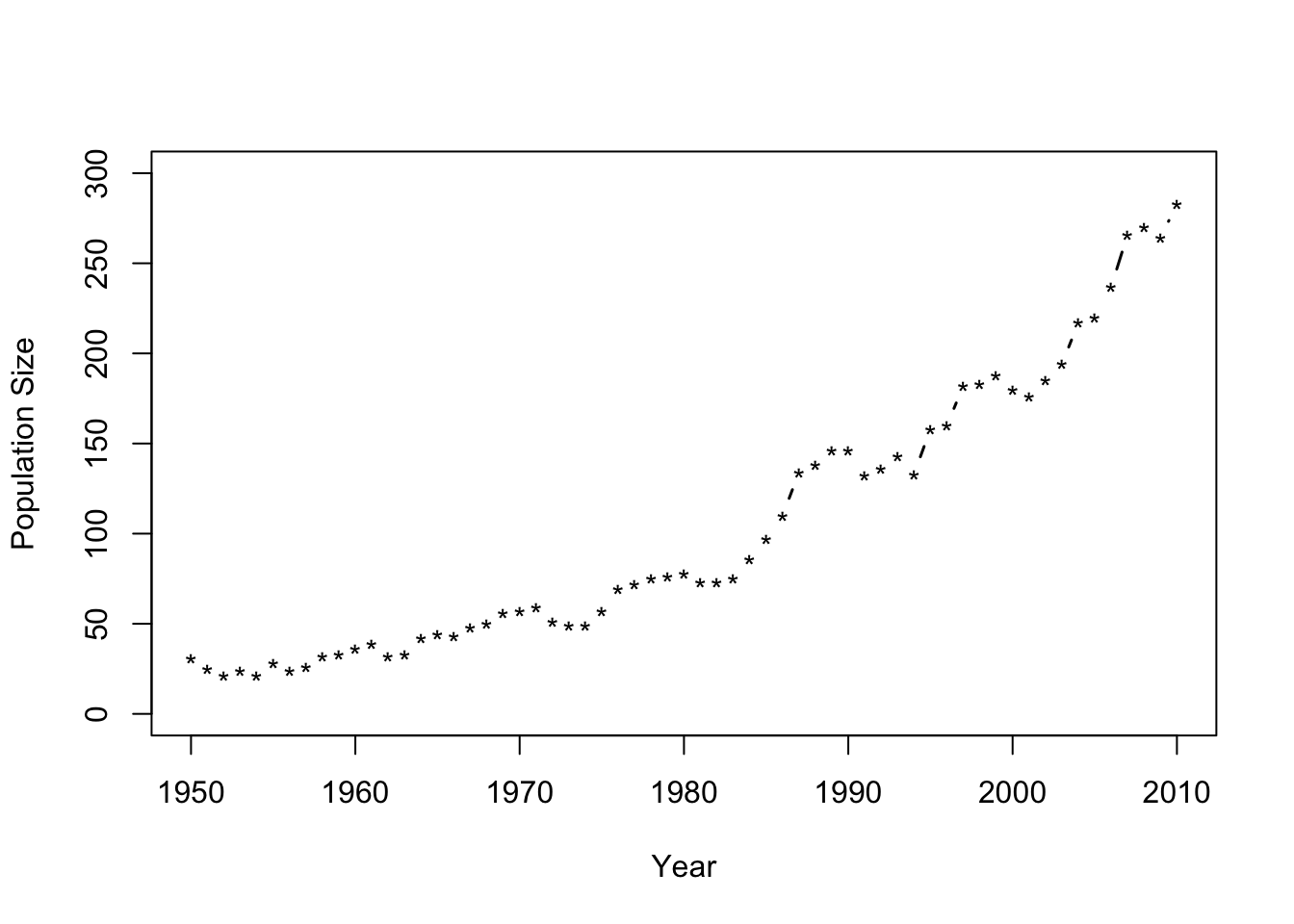
- Fit the model \(\mathbf{y}=\beta_{0}+\beta_{1}\mathbf{x}+\boldsymbol{\varepsilon}\) where \(\boldsymbol{\varepsilon}\sim\text{N}(\mathbf{0},\sigma^{2}\mathbf{I})\) and \(\mathbf{x}\) is the year.
m1 <- lm(N~Winter,data=df1)
plot(df1$Winter,df1$N,typ="b",xlab="Year",ylab="Population Size",ylim=c(0,300),lwd=1.5,pch="*")
abline(m1,col="gold")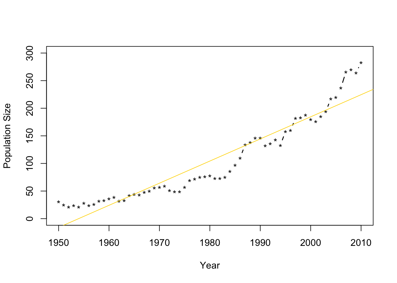
- Check model assumptions
e.hat <- residuals(m1)

#Check normality
hist(e.hat,col="grey",breaks=10,main="",xlab=expression(hat(epsilon)))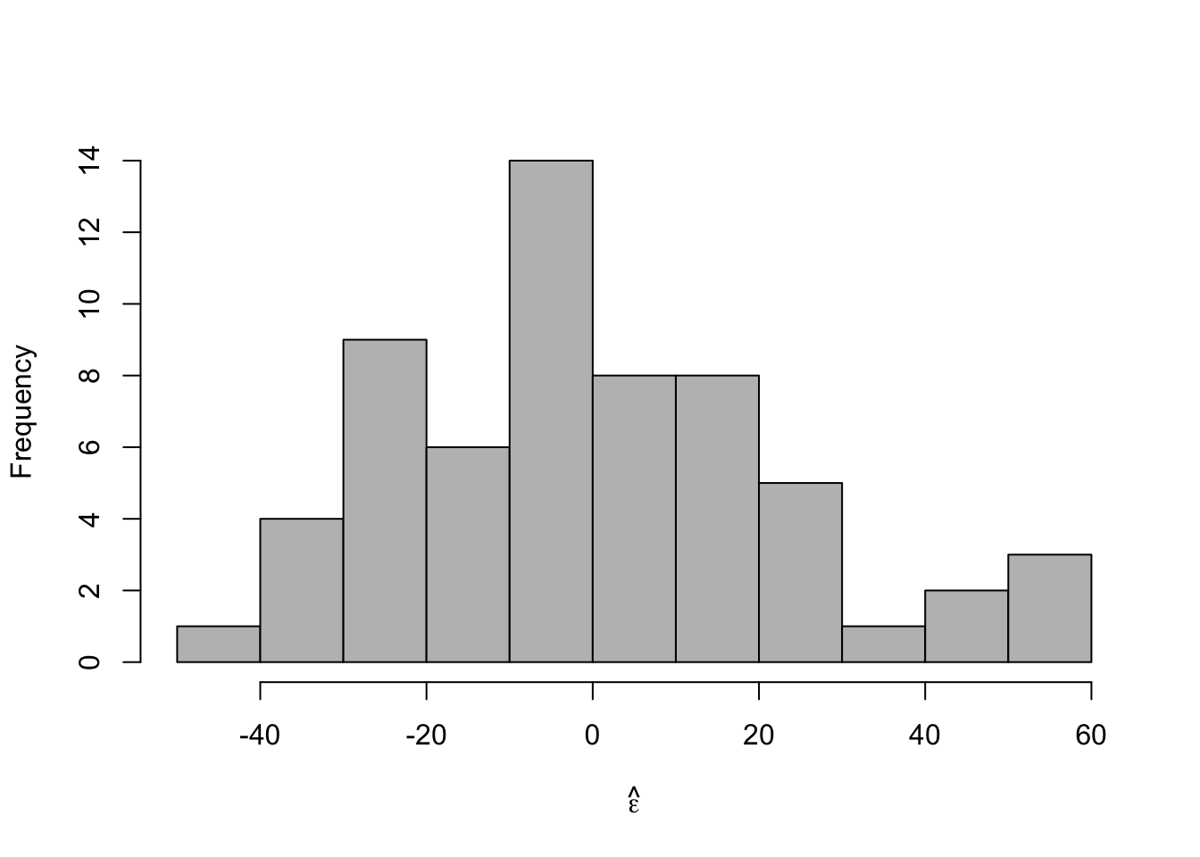
##
##  Shapiro-Wilk normality test
##
## data:  e.hat
## W = 0.96653, p-value = 0.09347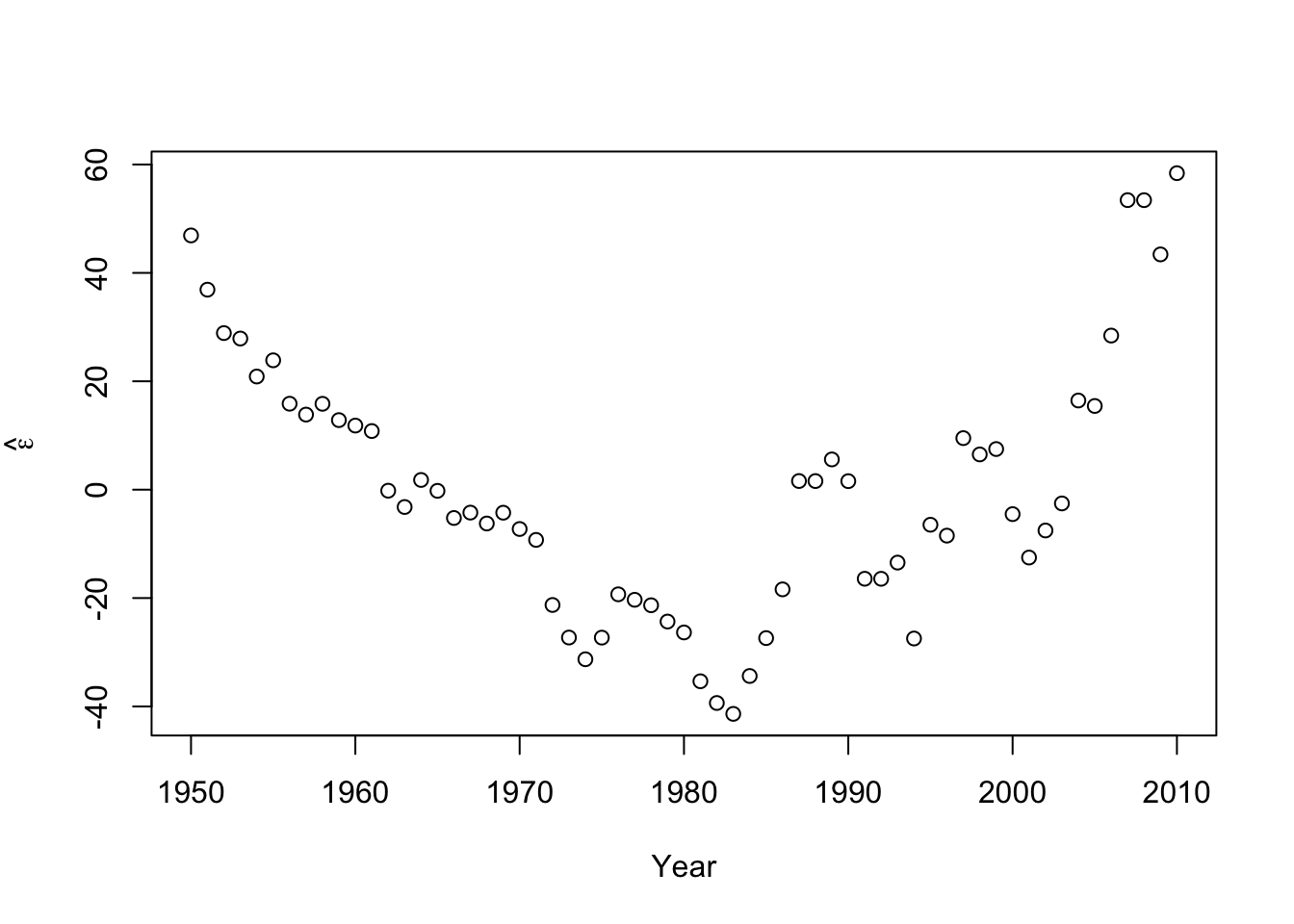
#Check for autocorrelation among residuals
plot(e.hat[1:60],e.hat[2:61],xlab=expression(hat(epsilon)[t]),ylab=expression(hat(epsilon)[t+1]))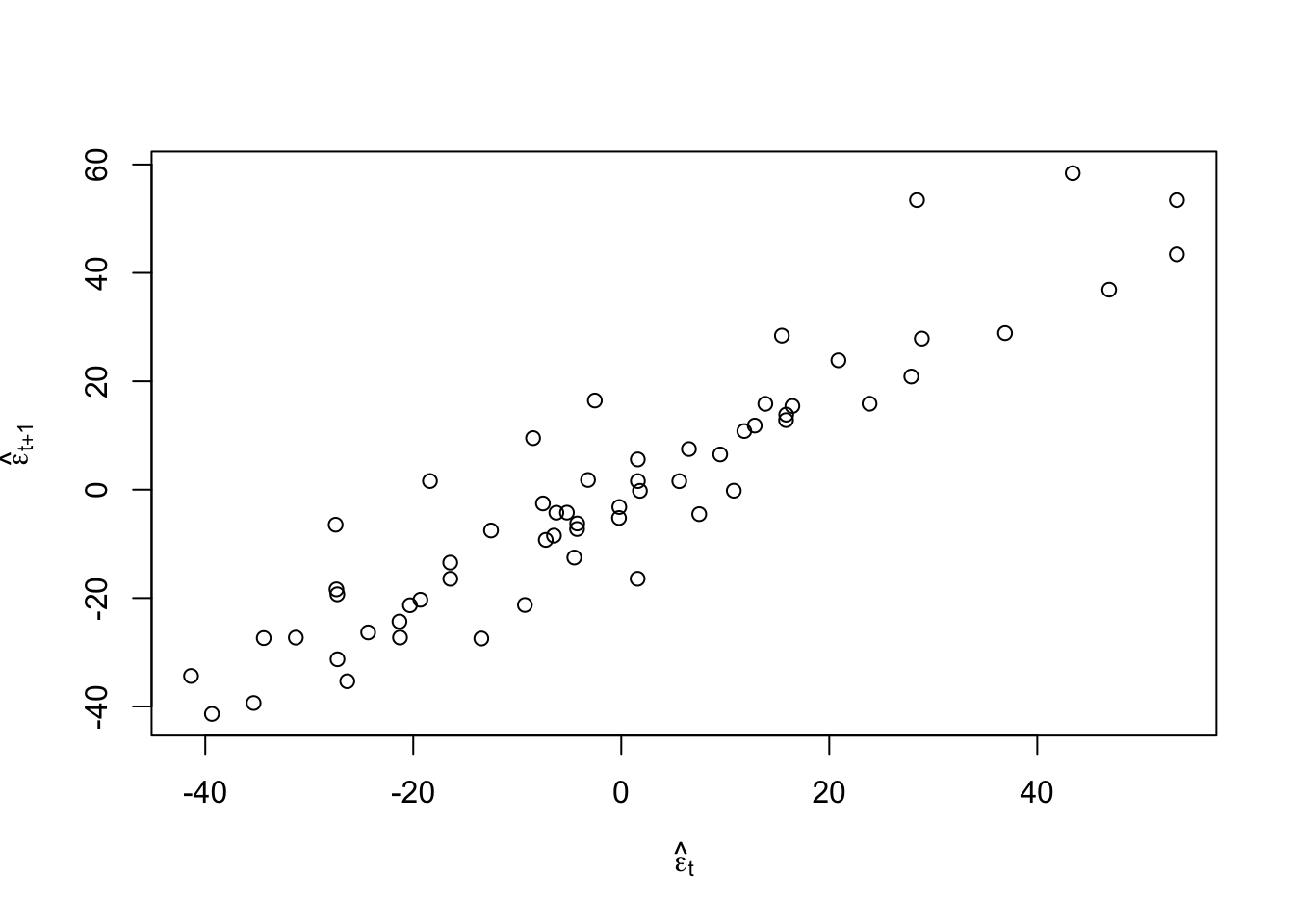
## [1] 0.9273559## ## Durbin-Watson test ## ## data: m1 ## DW = 0.13355, p-value < 2.2e-16 ## alternative hypothesis: true autocorrelation is greater than 0- Log transformation (i.e., \(\text{log}(\mathbf{y})\)).
- \(\text{log}(\mathbf{y})=\beta_{0}+\beta_{1}\mathbf{x}+\boldsymbol{\varepsilon}\) where \(\boldsymbol{\varepsilon}\sim\text{N}(\mathbf{0},\sigma^{2}\mathbf{I})\) and \(\mathbf{x}\) is the year.
- What model is implied by this transformation?
- If \(z\sim\text{N}(\mu,\sigma^{2})\), then \(\text{E}(e^{z})=e^{\mu+frac{\sigma^{2}}{2}}\) and \(\text{Var}(e^{z})=(e^{\sigma^{2}}-1)e^{2\mu+\sigma^{2}}\)
- Fit the model
m2 <- lm(log(N)~Winter,data=df1) plot(df1$Winter,df1$N,typ="b",xlab="Year",ylab="Population Size",ylim=c(0,300),lwd=1.5,pch="*") abline(m1,col="gold") ev.y.hat <- exp(predict(m2)) # Possible because of invariance property of MLEs points(df1$Winter,ev.y.hat,typ="l",col="deepskyblue")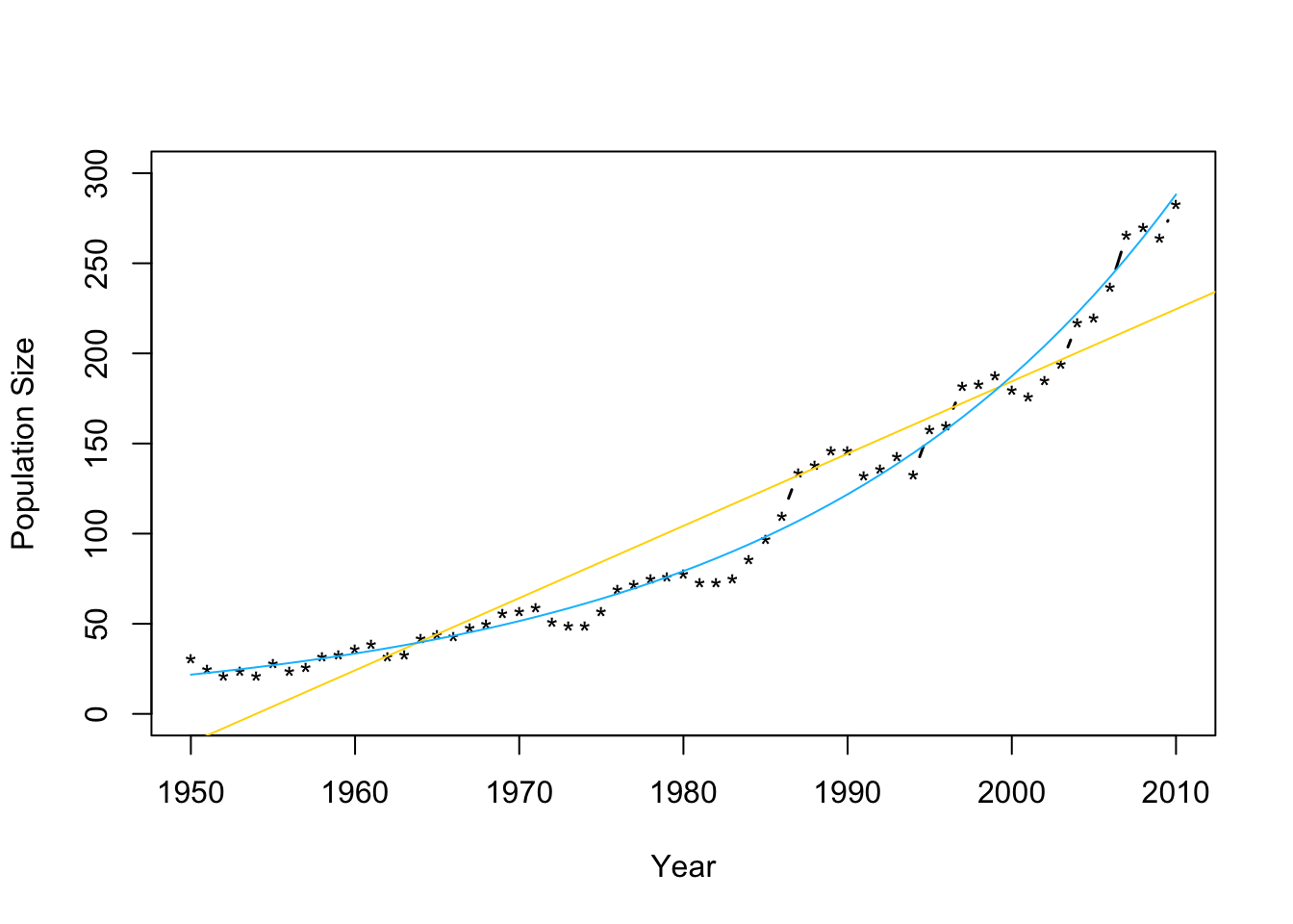 - Check model assumptions
e.hat <- residuals(m2)

#Check normality
hist(e.hat,col="grey",breaks=10,main="",xlab=expression(hat(epsilon)))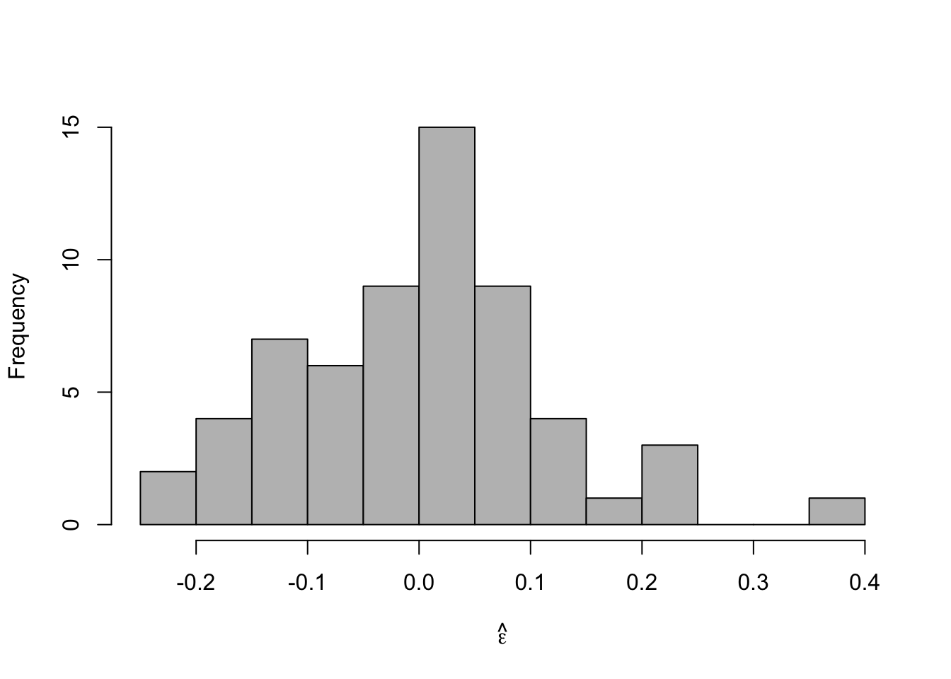
## ## Shapiro-Wilk normality test ## ## data: e.hat ## W = 0.97059, p-value = 0.1489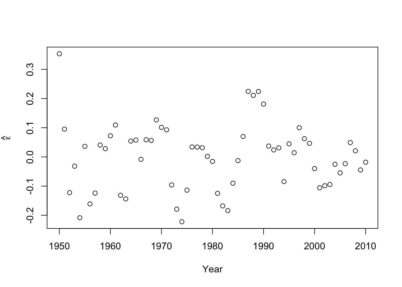 - Confidence intervals and prediction intervals
plot(df1$Winter,df1$N,typ="b",xlab="Year",ylab="Population Size",ylim=c(0,300),lwd=1.5,pch="*")
ev.y.hat <- exp(predict(m2)) # Possible because of invariance property of MLEs
points(df1$Winter,ev.y.hat,typ="l",col="deepskyblue")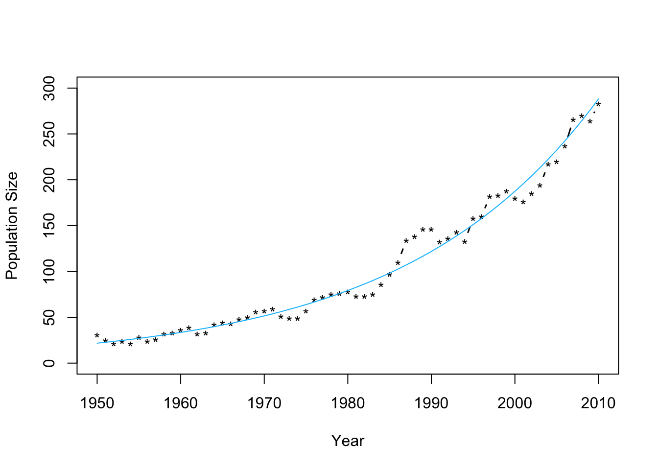
## fit lwr upr ## 1 3.080718 3.0223 3.139136## fit lwr upr ## 1 3.080718 2.842504 3.318933
Literature cited
Gelman, Andrew, Jessica Hwang, and Aki Vehtari. 2014. “Understanding Predictive Information Criteria for Bayesian Models.” Statistics and Computing 24 (6): 997–1016.