28 Day 28 (July 15)
28.1 Announcements
Please email me and request a 20 min time period during the final week of class (July 22 - 26) to give your final presentation. When you email me please suggest three times/dates that work for you.
Read Ch. 7 and 8 in linear models with R
28.2 Linear models for correlated errors
Motivating example
ISIT <- read.table("https://www.dropbox.com/scl/fi/4ycv4lp9f1kvfkkzdqpqo/bioluminescence.txt?rlkey=ebtdpismrkkxia0zo43svgusn&dl=1", header = TRUE)

Sources16 <- ISIT$Sources[ISIT$Station == 16]
Depth16 <- ISIT$SampleDepth[ISIT$Station == 16]
Sources16 <- Sources16[order(Depth16)]
Depth16 <- sort(Depth16)
plot(Depth16, Sources16, las = 1, ylim = c(0, 65), col = rgb(0, 0, 0, 0.25),
pch = 19)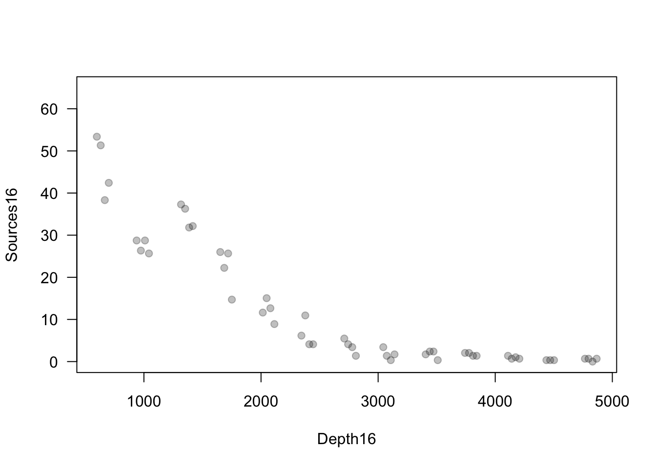
Linear model with correlated errors
- \(\mathbf{\textbf{y}}=\mathbf{X}\boldsymbol{\beta}+\boldsymbol{\eta}+\boldsymbol{\varepsilon}\) where \(\boldsymbol{\eta}\sim\text{N}(\mathbf{0},\sigma_{\eta}^{2}\mathbf{R}(\phi))\) and \(\boldsymbol{\varepsilon}\sim\text{N}(\mathbf{0},\sigma_{\varepsilon}^{2}\mathbf{I})\)
- The model above is the same as \(\mathbf{y}\sim\text{N}(\mathbf{X}\boldsymbol{\beta},\sigma_{\eta}^{2}\mathbf{R}(\phi)+\sigma^{2}\mathbf{I})\)
- Estimation
- Regression coefficients \[\hat{\boldsymbol{\beta}}=(\mathbf{X}^{\prime}\mathbf{V}^{-1}\mathbf{X})^{-1}\mathbf{X}^{\prime}\mathbf{V}^{-1}\mathbf{y}\] where \(\mathbf{V=}\sigma_{\eta}^{2}\mathbf{R}(\phi)+\sigma_{\varepsilon}^{2}\mathbf{I}\)
- Numerical maximization to estimate \(\sigma_{\eta}^{2}\), \(\sigma^{2}\), and \(\phi\)
- Error terms \[\hat{\boldsymbol{\eta}}=\hat{\sigma}_{\eta}^{2}\mathbf{R}(\hat{\phi})(\hat{\sigma}_{\varepsilon}^{2}\mathbf{I}+\hat{\sigma}_{\eta}^{2}\mathbf{R}(\hat{\phi}))^{-1}(\mathbf{y}-\mathbf{X}\hat{\boldsymbol{\beta}})\] \[\hat{\boldsymbol{\varepsilon}} = \mathbf{y} - \mathbf{X}\hat{\boldsymbol{\beta}} - \hat{\boldsymbol{\eta}}\]
Bioluminescence example
- Intercept only linear model
ISIT <- read.table("https://www.dropbox.com/scl/fi/4ycv4lp9f1kvfkkzdqpqo/bioluminescence.txt?rlkey=ebtdpismrkkxia0zo43svgusn&dl=1", header = TRUE)

Sources16 <- ISIT$Sources[ISIT$Station == 16]
Depth16 <- ISIT$SampleDepth[ISIT$Station == 16]
Sources16 <- Sources16[order(Depth16)]
Depth16 <- sort(Depth16)

m1 <- lm(Sources16~1)
e.hat.m1 <- residuals(m1)

plot(Depth16, e.hat.m1,
 xlab="Depth (m)",ylab=expression(hat(epsilon)),ylim=c(-15,60),las=1,col=rgb(0,0,0,0.25))
abline(a=0,b=0)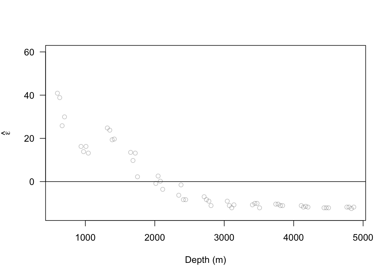
- Intercept only linear model with spatial random effect
library(nlme)
m2 <- gls(Sources16~1,correlation=corGaus(form=~Depth16,nugget=TRUE,value=c(100,0.05),fixed=FALSE),method="ML")

summary(m2)
## Generalized least squares fit by maximum likelihood ## Model: Sources16 ~ 1 ## Data: NULL ## AIC BIC logLik ## 296.3003 304.0276 -144.1502 ## ## Correlation Structure: Gaussian spatial correlation ## Formula: ~Depth16 ## Parameter estimate(s): ## range nugget ## 610.73574394 0.01300607 ## ## Coefficients: ## Value Std.Error t-value p-value ## (Intercept) 17.73824 8.981483 1.974978 0.0538 ## ## Standardized residuals: ## Min Q1 Med Q3 Max ## -0.8937320 -0.8247052 -0.6866517 0.3991341 1.7952883 ## ## Residual standard error: 19.84738 ## Degrees of freedom: 51 total; 50 residual# estimated range & nugget parameters from gls phi <- exp(m2$model[1]$corStruct[1])^2 nugget <- 1/(1+exp(-m2$model[1]$corStruct[2])) X <- rep(1,length(Sources16)) y <- Sources16 sigma2.eta <- (m2$sigma^2)*(1-nugget) R <- exp(-as.matrix(dist(Depth16,diag=TRUE,upper=TRUE))^2/phi) sigma2.e <- (m2$sigma^2)*nugget I <- diag(1,length(y)) V <- sigma2.eta*R + sigma2.e*I beta <- solve(t(X)%*%solve(V)%*%X)%*%t(X)%*%solve(V)%*%y eta <- sigma2.eta*R%*%solve(V)%*%(y-X%*%beta) par(mar=c(5.1,4.1,2.1,2.1),oma=c(0,0,0,0)) # reset plot margins par(mfrow=c(1,2)) # plot layout par(pch=19) # plotting symbol # plot predictions for second-order spatial model plot(Depth16, Sources16, xlab="Depth (m)",ylab="Sources",ylim=c(-15,60),las=1,col=rgb(0,0,0,0.25)) lines(Depth16,X%*%beta + eta,col="black") lines(Depth16,X%*%beta,col="purple") e.hat.m2 <- y - (X%*%beta + eta) plot(Depth16, e.hat.m2, xlab="Depth (m)",ylab=expression(hat(epsilon)),las=1,col=rgb(0,0,0,0.25))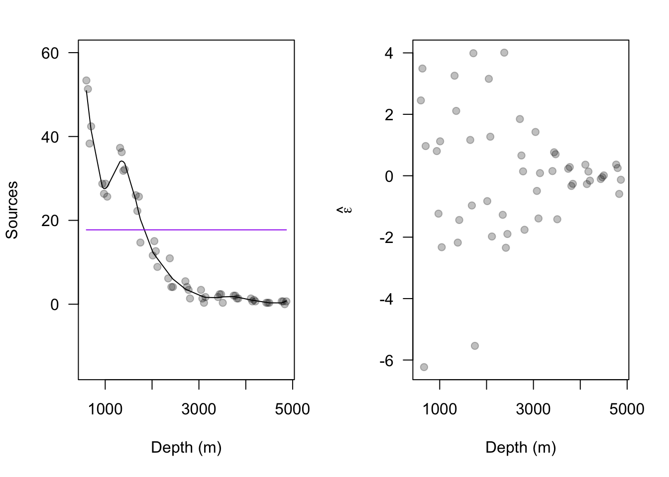
28.3 Collinearity
When two or more of the predictor variables (i.e., columns of \(\mathbf{X}\)) are correlated, the predictors are said to be collinear. Also called
- Collinearity
- Multicollinearity
- Correlation among predictors/covariates
- Partial parameter identifiability
Collinearity cause coefficient estimates (i.e., \(\hat{\boldsymbol{\beta}}\) to change when a collinear predictor is removed (or added) to the model.
- Extremely common problem with observational data and data collected from poorly designed experiments.
Example
- The data
library(httr)
library(readxl)

url <- "https://doi.org/10.1371/journal.pone.0148743.s005"
GET(url, write_disk(path <- tempfile(fileext = ".xls")))
df1 <- read_excel(path=path,sheet = "Data", col_names=TRUE,col_types="numeric") notes <- read_excel(path=path,sheet = "Notes", col_names=FALSE)## # A tibble: 6 × 9 ## States Year CDEP WKIL WPOP BRPA NCAT SDEP NSHP ## <dbl> <dbl> <dbl> <dbl> <dbl> <dbl> <dbl> <dbl> <dbl> ## 1 1 1987 6 4 10 2 9736 10 1478 ## 2 1 1988 0 0 14 1 9324 0 1554 ## 3 1 1989 3 1 12 1 9190 0 1572 ## 4 1 1990 5 1 33 3 8345 0 1666 ## 5 1 1991 2 0 29 2 8733 2 1639 ## 6 1 1992 1 0 41 4 9428 0 1608## # A tibble: 9 × 2 ## ...1 ...2 ## <chr> <chr> ## 1 Year <NA> ## 2 State 1=Montana,2=Wyoming,3=Idaho ## 3 Cattle depredated CDEP ## 4 Sheep depredated SDEP ## 5 Wolf population WPOP ## 6 Wolves killed WKIL ## 7 Breeding pairs BRPA ## 8 Number of cattleA* NCAT ## 9 Number of SheepB* NSHPFit a linear model
## ## Call: ## lm(formula = CDEP ~ NCAT + WPOP, data = df1) ## ## Residuals: ## Min 1Q Median 3Q Max ## -40.289 -8.147 -3.475 2.678 92.257 ## ## Coefficients: ## Estimate Std. Error t value Pr(>|t|) ## (Intercept) -3.8455597 8.1697216 -0.471 0.64 ## NCAT 0.0009372 0.0010363 0.904 0.37 ## WPOP 0.1031119 0.0119644 8.618 7.51e-12 *** ## --- ## Signif. codes: 0 '***' 0.001 '**' 0.01 '*' 0.05 '.' 0.1 ' ' 1 ## ## Residual standard error: 20.23 on 56 degrees of freedom ## (3 observations deleted due to missingness) ## Multiple R-squared: 0.5855, Adjusted R-squared: 0.5707 ## F-statistic: 39.55 on 2 and 56 DF, p-value: 1.951e-11- Killing wolves should reduce the number of cattle depredated, right? Let’s add the number of wolves killed to our model.
## ## Call: ## lm(formula = CDEP ~ NCAT + WPOP + WKIL, data = df1) ## ## Residuals: ## Min 1Q Median 3Q Max ## -18.519 -8.549 -1.588 4.049 79.041 ## ## Coefficients: ## Estimate Std. Error t value Pr(>|t|) ## (Intercept) 13.901373 6.511267 2.135 0.0372 * ## NCAT -0.001385 0.000830 -1.669 0.1008 ## WPOP 0.011868 0.015724 0.755 0.4536 ## WKIL 0.683946 0.097769 6.996 3.84e-09 *** ## --- ## Signif. codes: 0 '***' 0.001 '**' 0.01 '*' 0.05 '.' 0.1 ' ' 1 ## ## Residual standard error: 14.85 on 55 degrees of freedom ## (3 observations deleted due to missingness) ## Multiple R-squared: 0.7807, Adjusted R-squared: 0.7687 ## F-statistic: 65.25 on 3 and 55 DF, p-value: < 2.2e-16- What happened?!
##             WKIL       WPOP        NCAT
## WKIL  1.00000000  0.7933354 -0.04460099
## WPOP  0.79333543  1.0000000 -0.34440797
## NCAT -0.04460099 -0.3444080  1.00000000
Some analytical results
- Assume the linear model \[\mathbf{y}=\beta_{1}\mathbf{x}+\beta_{2}\mathbf{z}+\boldsymbol{\varepsilon}\] where \(\boldsymbol{\varepsilon}\sim\text{N}(\mathbf{0},\sigma^{2}\mathbf{I})\)
- Assume that the predictors \(\mathbf{x}\) and \(\mathbf{z}\) are correlated (i.e., are not orthogonal \(\mathbf{x}^{\prime}\mathbf{z}\neq 0\) and \(\mathbf{z}^{\prime}\mathbf{x}\neq 0\)).
- Then \[\hat{\beta}_1 = (\mathbf{x}^{\prime}\mathbf{x}\times\mathbf{z}^{\prime}\mathbf{z} - \mathbf{x}^{\prime}\mathbf{z}\times\mathbf{z}^{\prime}\mathbf{x})^{-1}((\mathbf{z}^{\prime}\mathbf{z})\mathbf{x}^{\prime} - (\mathbf{x}^{\prime}\mathbf{z})\mathbf{z}^{\prime})\mathbf{y}\] and \[\hat{\beta}_2 = (\mathbf{z}^{\prime}\mathbf{z}\times\mathbf{x}^{\prime}\mathbf{x} - \mathbf{z}^{\prime}\mathbf{x}\times\mathbf{x}^{\prime}\mathbf{z})^{-1}((\mathbf{x}^{\prime}\mathbf{x})\mathbf{z}^{\prime} - (\mathbf{z}^{\prime}\mathbf{x})\mathbf{x}^{\prime})\mathbf{y}.\] The variance is \[\text{Var}(\hat{\beta}_{1})=\sigma^{2}\bigg{(}\frac{1}{1-R^{2}_{xz}}\bigg{)}\frac{1}{\sum_{i=1}^{n}(x_{i}-\bar{x})^{2}}\] \[\text{Var}(\hat{\beta}_{2})=\sigma^{2}\bigg{(}\frac{1}{1-R^{2}_{xz}}\bigg{)}\frac{1}{\sum_{i=1}^{n}(z_{i}-\bar{z})^{2}}\]where \(R^{2}_{xz}\) is the correlation between \(\mathbf{x}\) and \(\mathbf{z}\) (see pg. 107 in Faraway (2014)).
Take away message
- \(\hat{\beta}_i\) is the unbiased and minimum variance estimator assuming all predictors for \(\beta_i \neq 0\) are in the model.
- \(\hat{\beta}_i\) depends on the other predictors in the model.
- Correlation among predictors increases the variance of \(\hat{\beta}_i\).
- Known as the variance inflation factor
- Collinearity is ubiquitous in any model with correlated predictors
##     NCAT     WPOP     WKIL
## 1.350723 3.637257 3.212207
Literature cited
Faraway, J. J. 2014. Linear Models with r. CRC Press.