25 Day 25 (July 10)
25.1 Announcements
- Next read Ch. 6 (Model diagnostics) in Linear models with R
- Grades are up to date
- Assignment 4 is posted and due Wednesday July 17
- In-class workday tomorrow
25.2 Model checking
- Model diagnostics (Ch 6 in Faraway (2014)) is a set of tools and procedures to see if the assumptions of our model are approximately correct.
- Statistical tests (e.g., Shapiro-Wilk test for normality)
- Specific
- What if you reject the null?
- Graphical
- Broad
- Subjective
- Widely used
- Predictive model checks
- More common for Bayesian models (e.g., posterior predictive checks)
- Statistical tests (e.g., Shapiro-Wilk test for normality)
- We will explore numerous ways to check
- Distributional assumptions
- Normality
- Constant variance
- Correlation among errors
- Detection of outliers
- Deterministic model structure
- Is \(\mathbf{X}\boldsymbol{\beta}\) a reasonable assumption?
- Distributional assumptions
25.3 Distributional assumptions
Why did we assume \(\mathbf{y}\sim\text{N}(\mathbf{X\boldsymbol{\beta}},\sigma^{2}\mathbf{I})\)?
Is the assumption \(\mathbf{y}\sim\text{N}(\mathbf{X\boldsymbol{\beta}},\sigma^{2}\mathbf{I})\) ever correct? Is there a “true” model?
When would we expect the assumption \(\mathbf{y}\sim\text{N}(\mathbf{X\boldsymbol{\beta}},\sigma^{2}\mathbf{I})\) to be approximately correct?
- Human body weights
- Stock prices
- Temperature
- Proportion of votes for a candidate in an elections
Checking distributional assumptions
- If \(\mathbf{y}\sim\text{N}(\mathbf{X\boldsymbol{\beta}},\sigma^{2}\mathbf{I})\), then \(\mathbf{y} - \mathbf{X\boldsymbol{\beta}}\sim ?\)
If the assumption \(\mathbf{y}\sim\text{N}(\mathbf{X\boldsymbol{\beta}},\sigma^{2}\mathbf{I})\) is approximately correct, then what should \(\hat{\boldsymbol{\varepsilon}}\) look like?
Example: checking the assumption that \(\boldsymbol{\varepsilon}\sim\text{N}(\mathbf{0},\sigma^{2}\mathbf{I})\)
- Data
y <- c(63, 68, 61, 44, 103, 90, 107, 105, 76, 46, 60, 66, 58, 39, 64, 29, 37,
27, 38, 14, 38, 52, 84, 112, 112, 97, 131, 168, 70, 91, 52, 33, 33, 27,
18, 14, 5, 22, 31, 23, 14, 18, 23, 27, 44, 18, 19)
year <- 1965:2011
df <- data.frame(y = y, year = year)

plot(x = df$year, y = df$y, xlab = "Year", ylab = "Annual count", main = "",
col = "brown", pch = 20)
m1 <- lm(y ~ year, data = df)
abline(m1)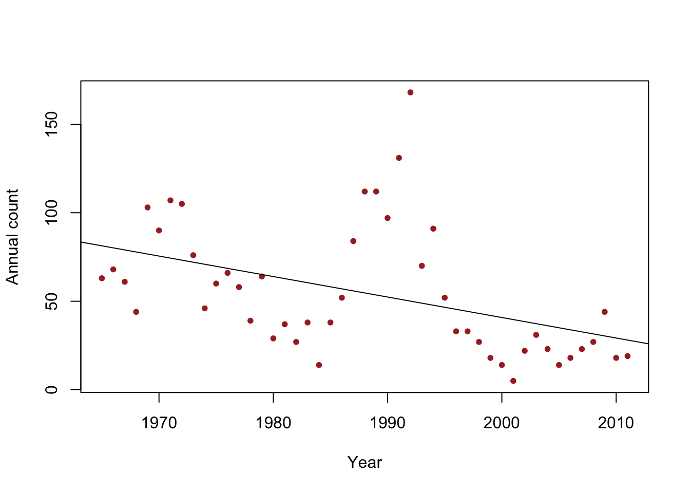
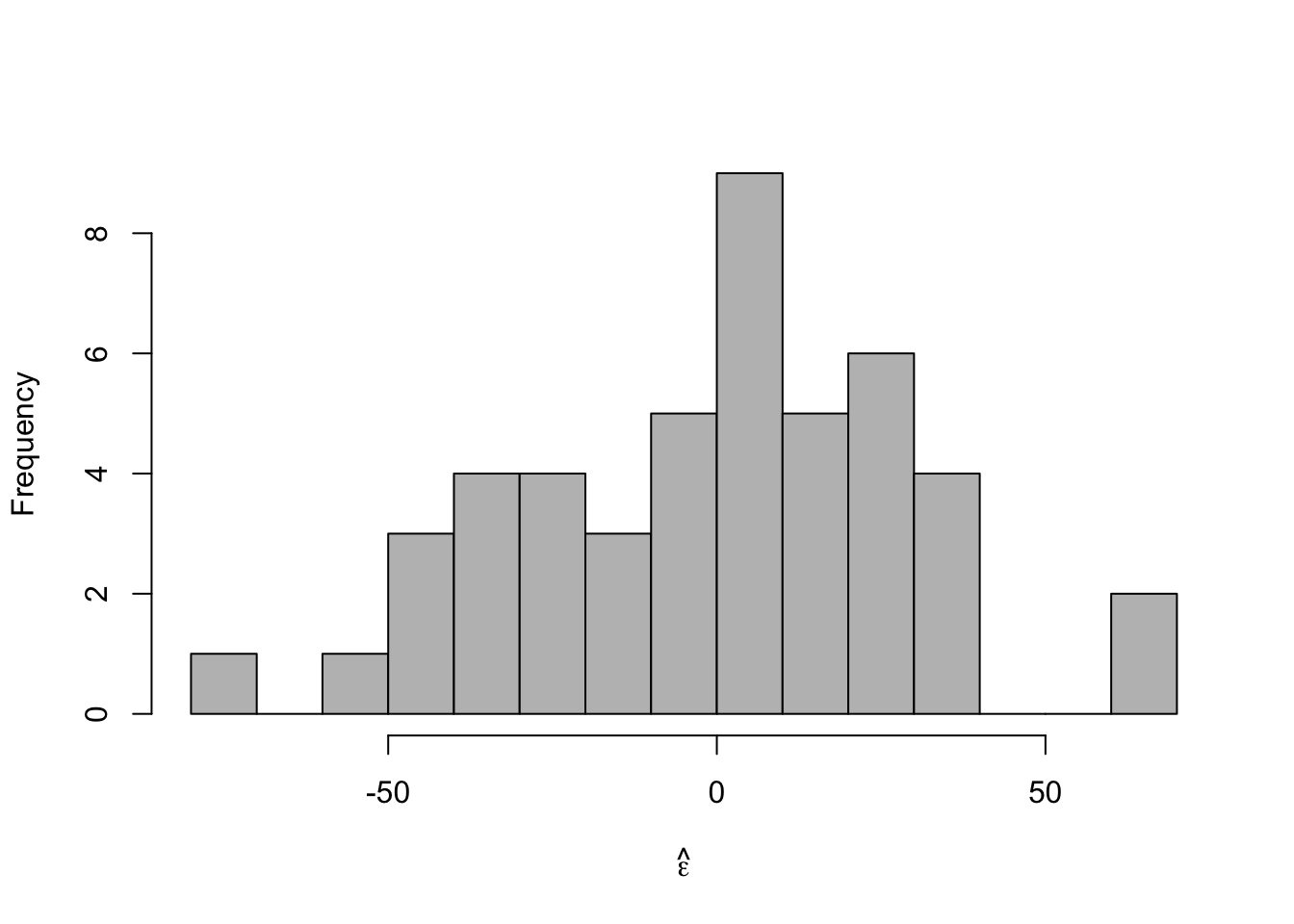
- Histogram of \(\hat{\boldsymbol{\varepsilon}}\)
m1 <- lm(y ~ year, data = df)
e.hat <- residuals(m1)
hist(e.hat,col="grey",breaks=15,main="",xlab=expression(hat(epsilon)))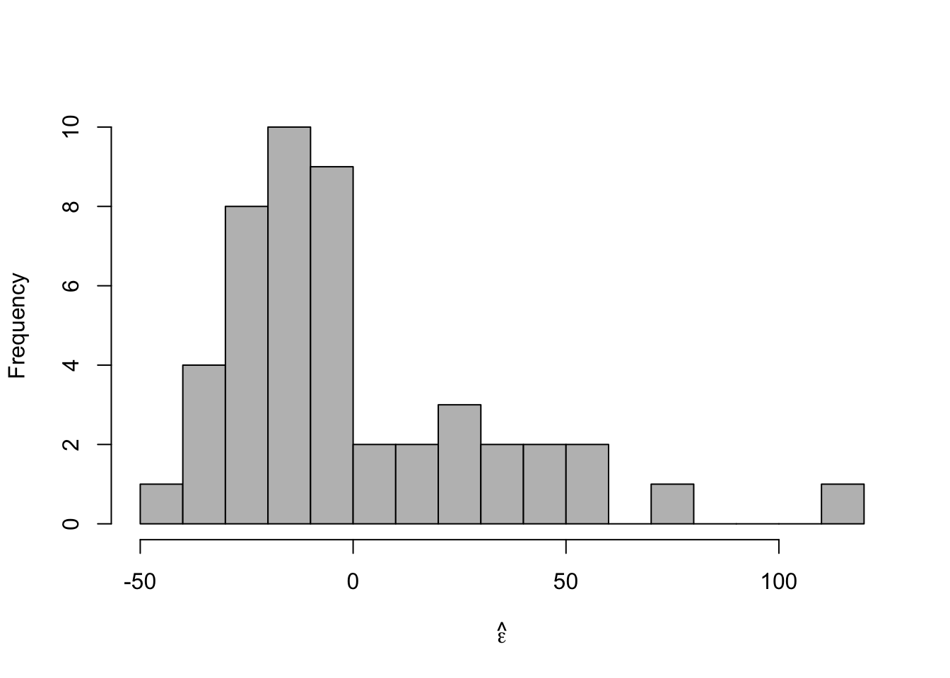
- Plot covariate vs. \(\hat{\boldsymbol{\varepsilon}}\)
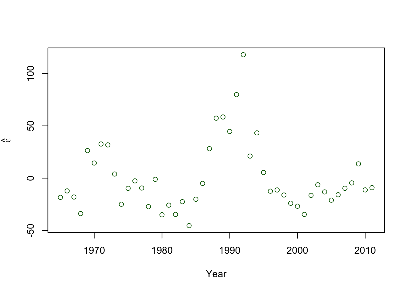
- A formal hypothesis test (see pg. 81 in Faraway (2014))
##
##  Shapiro-Wilk normality test
##
## data:  e.hat
## W = 0.86281, p-value = 5.709e-05
Example: Checking the assumption that \(\boldsymbol{\varepsilon}\sim\text{N}\left(\mathbf{0},\sigma^{2}\mathbf{I}\right)\) (What it should look like)
- Simulated data
beta.truth <- c(2356,-1.15)
sigma2.truth <- 33^2
n <- 47


year <- 1965:2011
X <- model.matrix(~year)
set.seed(2930)
y <- rnorm(n,X%*%beta.truth,sigma2.truth^0.5)
df1 <- data.frame(y = y, year = year)

plot(x = df1$year, y = df1$y, xlab = "Year", ylab = "Annual count", main = "",
col = "brown", pch = 20)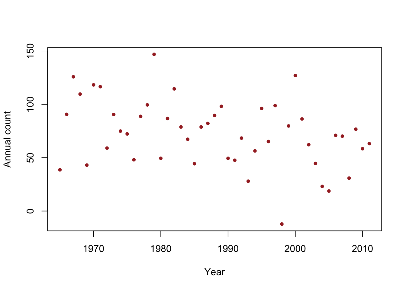
## ## Call: ## lm(formula = y ~ year, data = df1) ## ## Residuals: ## Min 1Q Median 3Q Max ## -76.757 -22.237 3.767 19.353 66.634 ## ## Coefficients: ## Estimate Std. Error t value Pr(>|t|) ## (Intercept) 1717.2121 638.5293 2.689 0.0100 * ## year -0.8272 0.3212 -2.575 0.0134 * ## --- ## Signif. codes: 0 '***' 0.001 '**' 0.01 '*' 0.05 '.' 0.1 ' ' 1 ## ## Residual standard error: 29.87 on 45 degrees of freedom ## Multiple R-squared: 0.1285, Adjusted R-squared: 0.1091 ## F-statistic: 6.632 on 1 and 45 DF, p-value: 0.01337- Histogram of \(\hat{\boldsymbol{\varepsilon}}\)
- Plot covariate vs. \(\hat{\boldsymbol{\varepsilon}}\)
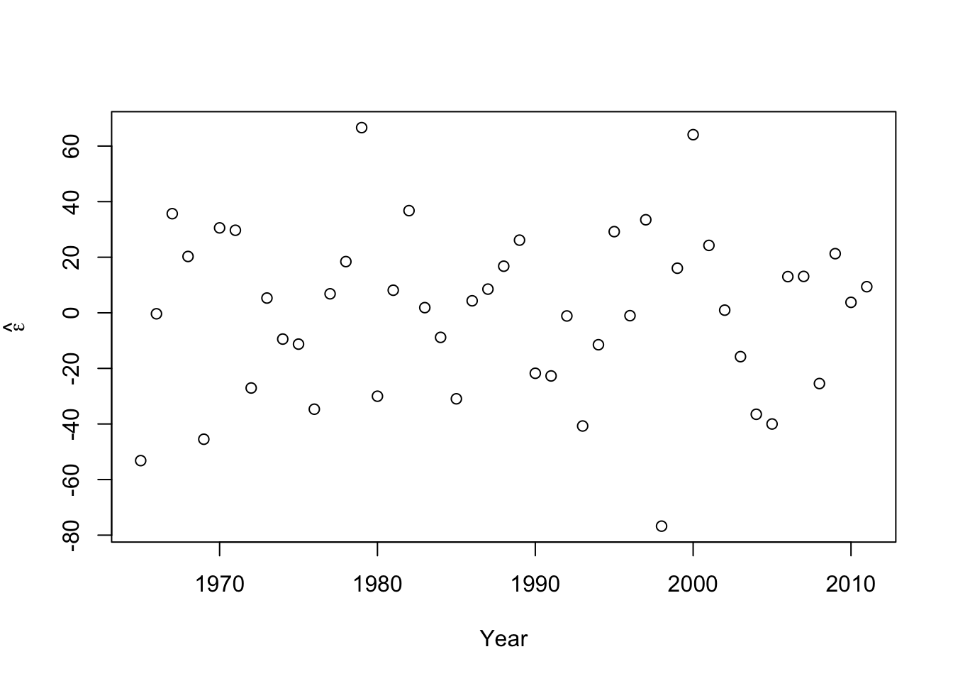
- A formal hypothesis test (see pg. 81 in Faraway (2014))
##
##  Shapiro-Wilk normality test
##
## data:  e.hat
## W = 0.98556, p-value = 0.8228