C Quick Start Guide
C.1 Reading in Data
See also Section 3.2.
Imagine that we have two files with financial data, a comma-separated values (csv) file called nasdaq_fundamentals.csv and an Excel workbook called s&p500.xlsx. To read these files into R, we need to:
- Load the appropriate package.
- Note the directory on our machine where these files are stored.
- Use the appropriate function to read in the data from the file location.
C.1.1 CSV Files
First let’s read in the data from the csv file, which contains metrics pulled from company 10K fillings.
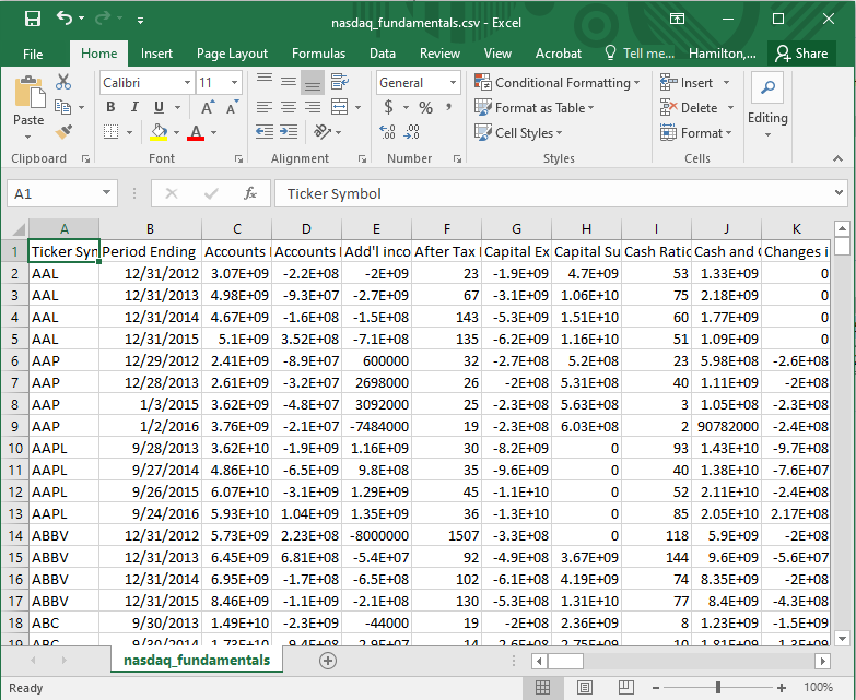
Figure C.1: nasdaq_fundamentals.csv.
Suppose this file were stored in the folder C:\reading_data. To read it into R, we do the following:
- Load the
tidyverse. - Store the full path to the file in a variable called
filePath. Note that our file path needs to use forward slashes (/) to separate subdirectories. - Read the data in from
filePathusing theread_csv()function from thetidyverse.
# Step 1
library(tidyverse)

# Step 2
filePath <- "C:/reading_data/nasdaq_fundamentals.csv"

# Step 3
fundamentals <- read_csv(filePath)
C.1.2 Excel Workbooks
Now let’s read in the data from the Excel workbook, which contains information on different sectors of the S&P 500. Note that this Excel file contains multiple tabs, each representing a different sector. We start by reading in the data from the Utilities tab.
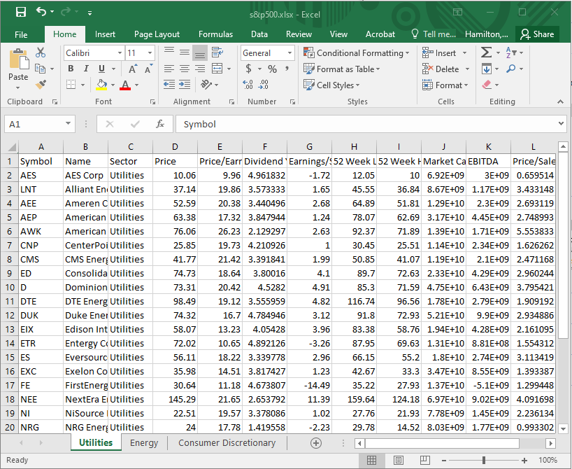
Figure C.2: s&p500.xlsx, Utilities tab.
To read this data into R, we follow similar steps as before, but this time use the read_excel() function from the readxl package:
- Load the
readxlpackage. - Store the full path to the file in a variable called
filePath. Note that our file path needs to use forward slashes (/) to separate subdirectories. - Read the data in from
filePathusing theread_excel()function from thereadxlpackage. Note that we use thesheetargument to specify the name of the tab in the Excel workbook that we want to read in.
# Step 1
library(readxl)

# Step 2
filePath <- "C:/reading_data/s&p500.xlsx"

# Step 3
utilities <- read_excel(filePath, sheet="Utilities")
Finally, let’s read in the data from the Energy tab of the Excel file.
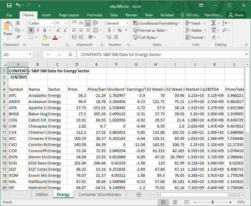
Figure C.3: s&p500.xlsx, Energy tab.
Note that this tab contains some extraneous text in the first few rows, and our data does not start until the fourth row. We account for this in Step 3 by specifying the range of cells in the file that contain the data of interest:
- Load the
readxlpackage. - Store the full path to the file in a variable called
filePath. Note that our file path needs to use forward slashes (/) to separate subdirectories. - Read the data in from
filePathusing theread_excel()function from thereadxlpackage. Note that we use thesheetargument to specify the name of the tab in the Excel workbook that we want to read in. To ignore the extraneous information at the top of the file, we have two options:- Set the
skipargument to3so that the first three rows of the file are ignored. - Set the
rangeargument to"A4:N36"so that only the data within that range is read in.
- Set the
# Step 1
library(readxl)

# Step 2
filePath <- "C:/reading_data/s&p500.xlsx"

# Step 3
utilities <- read_excel(filePath, sheet="Energy", skip=3)
# - OR -
utilities <- read_excel(filePath, sheet="Energy", range="A4:N36")
C.2 Linear Regression
See also Section 6.2.
Suppose we have a data frame called housing with real estate transaction data from Saratoga Springs, New York (ADD source: https://dasl.datadescription.com/datafile/saratoga-house-prices/). The first few observations of this data set are shown below.
| Price | Baths | Bedrooms | Fireplace | Acres | Age |
|---|---|---|---|---|---|
| 142.212 | 1.0 | 3 | 0 | 2.00 | 133 |
| 134.865 | 1.5 | 3 | 1 | 0.38 | 14 |
| 118.007 | 2.0 | 3 | 1 | 0.96 | 15 |
| 138.297 | 1.0 | 2 | 1 | 0.48 | 49 |
| 129.470 | 1.0 | 3 | 1 | 1.84 | 29 |
| 206.512 | 2.0 | 3 | 0 | 0.98 | 10 |
These variables are defined as follows:
Price: The sales price of a home in thousands of dollars.Baths: The number of bathrooms in the home.Bedrooms: The number of bedrooms in the home.Fireplace: Whether the home has a fireplace.Acres: The lot size in acres.Age: The age of the home in years.
We can fit a regression with Price as the dependent (\(Y\)) variable using the lm() function as follows:
fit <- lm(Price ~ Baths + Bedrooms + Fireplace + Acres + Age, data=housing)Then we can apply the summary() function to fit to get a summary of our model:
summary(fit)##
## Call:
## lm(formula = Price ~ Baths + Bedrooms + Fireplace + Acres + Age,
## data = housing)
##
## Residuals:
## Min 1Q Median 3Q Max
## -141.47 -33.43 -6.11 19.78 470.00
##
## Coefficients:
## Estimate Std. Error t value Pr(>|t|)
## (Intercept) -27.17190 8.61390 -3.154 0.001654 **
## Baths 65.38343 3.78293 17.284 < 0.0000000000000002 ***
## Bedrooms 16.92751 2.91667 5.804 0.00000000857 ***
## Fireplace 21.12512 4.27226 4.945 0.00000088638 ***
## Acres 8.78877 2.37834 3.695 0.000231 ***
## Age -0.04538 0.05945 -0.763 0.445458
## ---
## Signif. codes: 0 '***' 0.001 '**' 0.01 '*' 0.05 '.' 0.1 ' ' 1
##
## Residual standard error: 60.55 on 1057 degrees of freedom
## Multiple R-squared: 0.4887, Adjusted R-squared: 0.4863
## F-statistic: 202.1 on 5 and 1057 DF, p-value: < 0.00000000000000022We can apply confint() to fit() to get a 95% confidence interval for each of the coefficients of our model:
confint(fit)## 2.5 % 97.5 %
## (Intercept) -44.0741786 -10.26961652
## Baths 57.9605197 72.80634988
## Bedrooms 11.2043862 22.65062633
## Fireplace 12.7420535 29.50819039
## Acres 4.1219695 13.45558042
## Age -0.1620358 0.07127757Finally, to check that our error terms are normally-distributed, we can create a qq-plot by applying the plot() function with which=2 as a parameter:
plot(fit, which=2)
This qq-plot is problematic, as the right-hand side shows unusual tail behavior. This is likely because Price is positively-skewed; there are a handful of “outlier” houses that are very expensive. To address this, we could try fitting a new regression where we model the log of Price as our independent variable:
fitLog <- lm(log(Price) ~ Baths + Bedrooms + Fireplace + Acres + Age, data=housing)
plot(fitLog, which=2)
C.3 Estimating \(\beta\) of a Stock
To estimate the “beta” (\(\beta\)) of a stock:
- Load the
quantmodpackage. - Use the
getSymbols()function to pull the historical returns data for a particular stock over a given period. - Use
getSymbols()to pull the S&P 500 market returns data for the same time period. - Extract the returns from the objects created in steps 2 & 3.
- Use
lm()to regress the market returns onto the stock returns.
Following these steps, let’s calculate an estimate for the five-year monthly \(\beta\) on Disney at the time of writing (May 4, 2021). Note that “DIS” is the ticker for Disney and “SPY” is the ticker for the S&P 500.
# Step 1
library(quantmod)

# Step 2
DIS <- getSymbols("DIS", from="2016-05-04", to="2021-05-04", auto.assign=FALSE)

# Step 3
SPY <- getSymbols("SPY", from="2016-05-04", to="2021-05-04", auto.assign=FALSE)

# Step 4
disReturns <- monthlyReturn(Ad(DIS))
spyReturns <- monthlyReturn(Ad(SPY))

# Step 5
fit <- lm(disReturns ~ spyReturns)
summary(fit)
##
## Call:
## lm(formula = disReturns ~ spyReturns)
##
## Residuals:
## Min 1Q Median 3Q Max
## -0.07951 -0.04643 -0.01340 0.03205 0.18854
##
## Coefficients:
## Estimate Std. Error t value Pr(>|t|)
## (Intercept) -0.003560 0.007992 -0.445 0.658
## spyReturns 1.190924 0.178991 6.654 0.0000000104 ***
## ---
## Signif. codes: 0 '***' 0.001 '**' 0.01 '*' 0.05 '.' 0.1 ' ' 1
##
## Residual standard error: 0.05917 on 59 degrees of freedom
## Multiple R-squared: 0.4287, Adjusted R-squared: 0.419
## F-statistic: 44.27 on 1 and 59 DF, p-value: 0.00000001041Of course, it is important to note the 95% confidence interval on our estimate of \(\beta\), which we can get using confint():
confint(fit)## 2.5 % 97.5 %
## (Intercept) -0.01955259 0.01243256
## spyReturns 0.83276366 1.54908354