Chapter 9 Tool Tutorials
Some tools we will be using are:
kernel_densitycluster_points
When we load into R these specialty tools, we use the function load() instead of st_read() or library(). That’s because they were custom-written for this course as snippets of code. This saves you some effort down the road, and let’s you focus on the analysis part.
9.1 Kernel Density
9.1.1 What it does
Kernel density mapping is a technique to visualize the density of points on a map. In short, the technique takes a distance value (called a bandwidth) and calculates a density value for all points within that distance. It applies this across all points on map to generate ‘high’ and ‘low’ values of point density. In criminology we often use this as a visualization tool to help identify locations with high densities of crime over a given period of time. Depending on our problem and approach, we can then come up with a crime prevention strategy.
9.1.2 Walkthrough
# Load in libraries
library(sf)
library(tidyverse)

# Load data and import shapefiles
load("C:/Users/gioc4/Desktop/kernel_density.Rdata")

nh_city <- st_read("C:/Users/gioc4/Desktop/new_haven.shp")
nh_homicides <- st_read("C:/Users/gioc4/Desktop/nh_homicides.shp")
Let’s start by using the default measures in the kernel_density function. The minimum you need to specify is the name
of the point data and the name of the polygon data. Here, that’s nh_homicides and nh_city respectively. By default, kernel_density will try and give you a decent default bandwidth, but I will encourage you to apply real-world
knowledge to specify the bandwidth manually. Let’s take a look:
# Kernel density on NH homicides
# Save as an object named 'kde_homicide'

kde_homicide <- kernel_density(point_data = nh_homicides,
                               polygon_data = nh_city)
## Warning in showSRID(SRS_string, format = "PROJ", multiline = "NO", prefer_proj =
## prefer_proj): Discarded datum D_unknown in Proj4 definition## [1] "Calculating bandwith..."
## [1] "Bandwidth: 968.3"## Warning in showSRID(uprojargs, format = "PROJ", multiline = "NO", prefer_proj
## = prefer_proj): Discarded datum Unknown based on Clarke 1866 ellipsoid in Proj4
## definition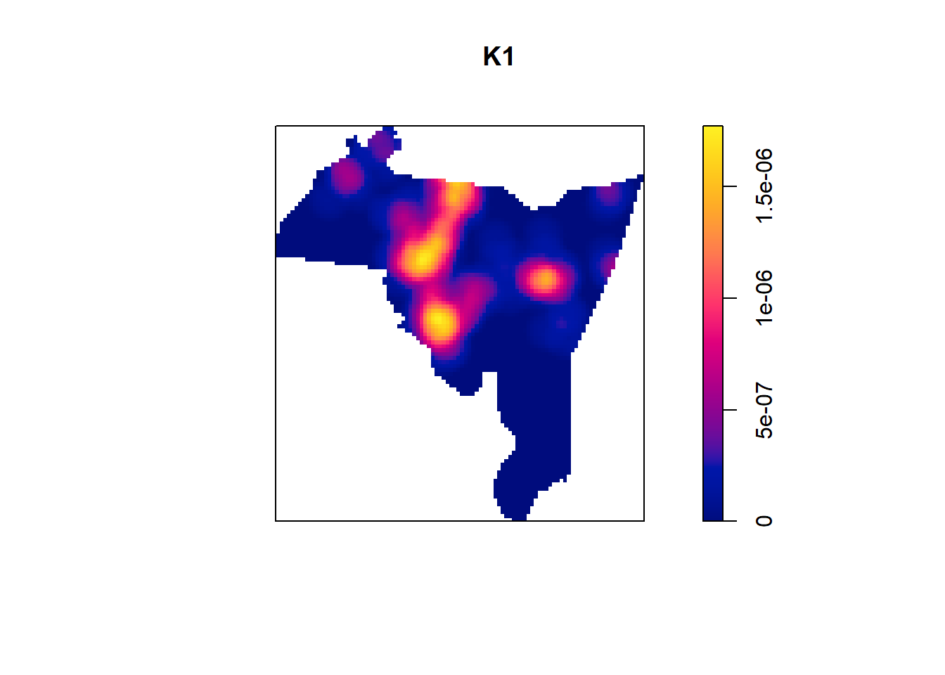
This gives us a preview of the plot and then saves the actual data into a variable that we called kde_homicide. We can
also see that the automatically calculated bandwidth was 943.3 feet, which seems reasonable.
The next logical step would be to take this data and use it to create a plot of our own. If we look at the data inside of that object, we will see three variables:
# Look at the top 6 rows of the kde object

head(kde_homicide)
## density X Y
## 1 2.214209e-07 542910.5 188261.5
## 2 1.859981e-07 543289.4 188261.5
## 3 1.716808e-07 543668.3 188261.5
## 4 3.823050e-07 542152.6 187855.4
## 5 3.571624e-07 542531.5 187855.4
## 6 3.174577e-07 542910.5 187855.4Where density is the kernel density value for each ‘cell’ on the map, and X and Y are the x-y coordinates for the
center of the ‘cell.’ We can plug this into ggplot to create our own map. All we have to do is use the function
geom_raster to create a raster object, then plug in the value that controls the color of each cell (which in this
case is the density value). We’ll use the default ggplot color theme, and use theme_void to get rid of
the background.
# Create a hot spot map in ggplot
# put in x-y coordinates an density inside the aes
# theme_void to remove background

ggplot() +
  geom_raster(data = kde_homicide, aes(x = X, y = Y, fill = density)) +
  theme_void()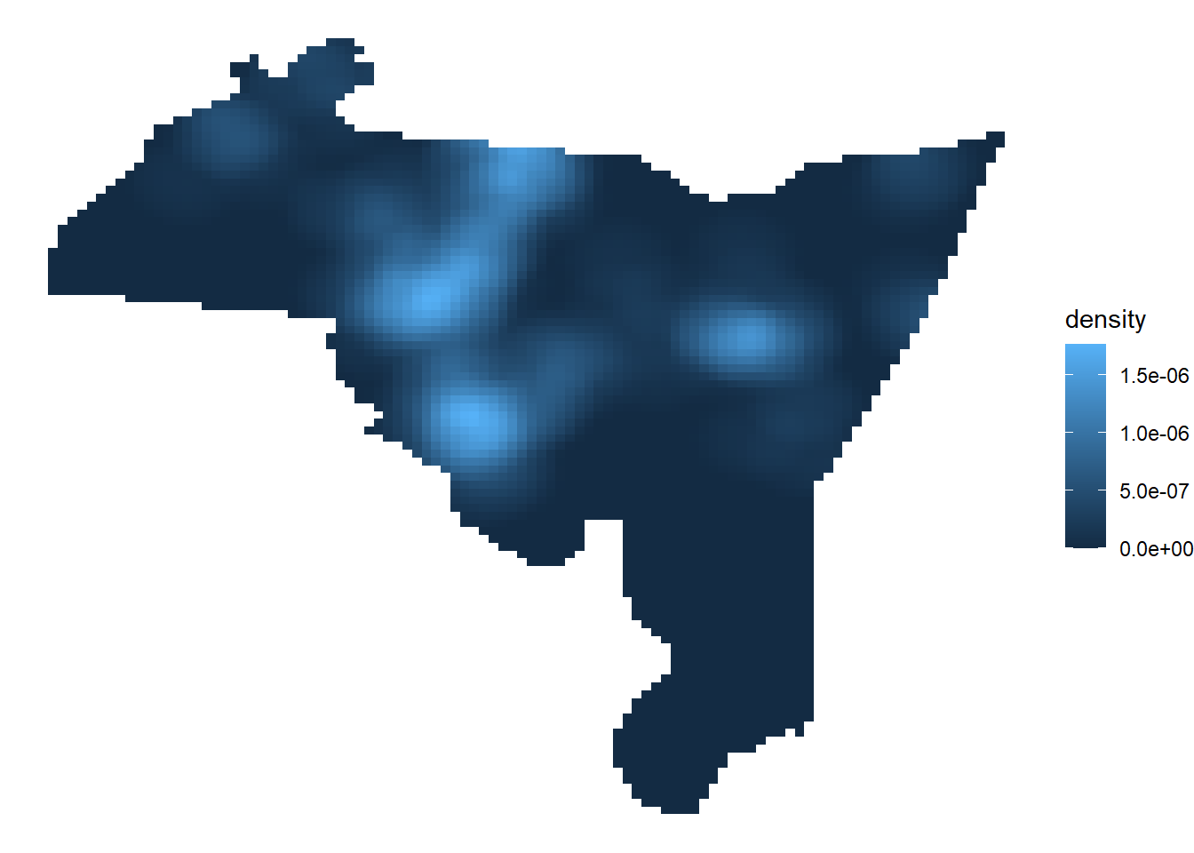
Finally, we can clean this up by adding the boundaries of New Haven, as well as adding in the points. We’ll also change
the color scheme to the viridis color as well. A finished map might look something like this below:
# Add boundaries of new haven, setting fill to NA
# Add title with labs
# scale_fill_viridis_c color scheme

ggplot() +
  geom_raster(data = kde_homicide, aes(x = X, y = Y, fill = density)) +
  geom_sf(data = nh_city, fill = NA, size = 1, color = 'black') +
  labs(title = "New Haven Homicides (2010 - 2019)") +
  scale_fill_viridis_c() +
  theme_void()
9.2 Cluster Points
9.2.1 What it does
cluster_points is a function that utilizes the dbscan function in R. dbscan is a:
Fast reimplementation of the DBSCAN (Density-based spatial clustering of applications with noise) clustering algorithm using a kd-tree.
Which means, more simply, is that it is a statistical approach to clustering points and separating out ‘noise.’ It is not uncommon to hundreds or even thousands of points with seemingly no pattern. We can rely on statistical methods to help us isolate patterns (signal) from the rest of the data (noise). We might use this to help us identify hot spot clusters, to come up with new patrol areas, or to use in a predictive analysis. See a paper by Wheeler and Reuter (2020) here.
9.2.2 Walkthrough
Let’s start by loading in the cluster_points function and the New Haven data. Remember, use load() to load in the
tools.
# Load in libraries
library(sf)
library(dbscan)
library(tidyverse)

# Load data and import shapefiles
load("C:/Users/gioc4/Desktop/cluster_points.Rdata")

nh_city <- st_read("C:/Users/gioc4/Desktop/new_haven.shp")
nh_homicides <- st_read("C:/Users/gioc4/Desktop/nh_homicides.shp")
Now that we’ve loaded the data in, let’s first plot everything out and evaluate our next steps. I’ll create a plot with the homicides as small red points, and the city of New Haven as the default grey background. Below we see the distribution of homicides in New Haven from 2010 through 2019. There are some obvious clusters, but also some overlap as well.
# Plot out city and homicides
ggplot() +
  geom_sf(data = nh_city) +
  geom_sf(data = nh_homicides, color = 'red', size = .6)
Let’s use the function cluster_points to help us identify clusters of points that are nearer to each other and are
in relatively uniform space. This will help us come up with some regions to identify as ‘hot spots’ where we might
employ some kind of initiative. The cluster_points function has a few arguments that you will need to adjust.
Below are the four most important ones:
point_data- The point feature you are clusteringpolygon_data- A polygon feature enclosing the pointspts- The minimum number of ‘core’ pointsdist- The maximum distance to search for points
Let’s start by running with the default settings (pts = 3, dist = 1000). The absolute minimum you need to
specify is what your point data is, and what your polygon data is. Take a look:
# Run cluster points with default settings
# Add 'plot = TRUE' to plot out automatically

cluster_points(point_data = nh_homicides,
               polygon_data = nh_city)
## DBSCAN clustering for 161 objects.
## Parameters: eps = 1000, minPts = 5
## The clustering contains 10 cluster(s) and 53 noise points.
##
## 0 1 2 3 4 5 6 7 8 9 10
## 53 9 17 21 19 12 6 5 5 9 5
##
## Available fields: cluster, eps, minPts
This gives us a few things. First we see that using the default measures we obtained 10 clusters. The largest cluster has 21 homicides, while the smallest has 5. The ‘noise’ points represent homicides that don’t belong to any cluster, based on our specifications. Looking at the map, some of the clusters are very, very small and adjacent to others. We can see the location of these clusters as well by looking at the legend on the right side listed 1 through 10.
Maybe we think that we should require more points for a cluster. Let’s try adjusting the value pts and dist.
Here, I’m going to specify that a cluster needs to have a minimum of 10 homicides that are within 1500 feet.
This should shrink the number of clusters, while increasing their size.
# Increase pts to 10
# dist to 1500

cluster_points(point_data = nh_homicides,
               polygon_data = nh_city,
               pts = 10,
               dist = 1500)
## DBSCAN clustering for 161 objects.
## Parameters: eps = 1500, minPts = 10
## The clustering contains 4 cluster(s) and 66 noise points.
##
## 0 1 2 3 4
## 66 14 29 40 12
##
## Available fields: cluster, eps, minPts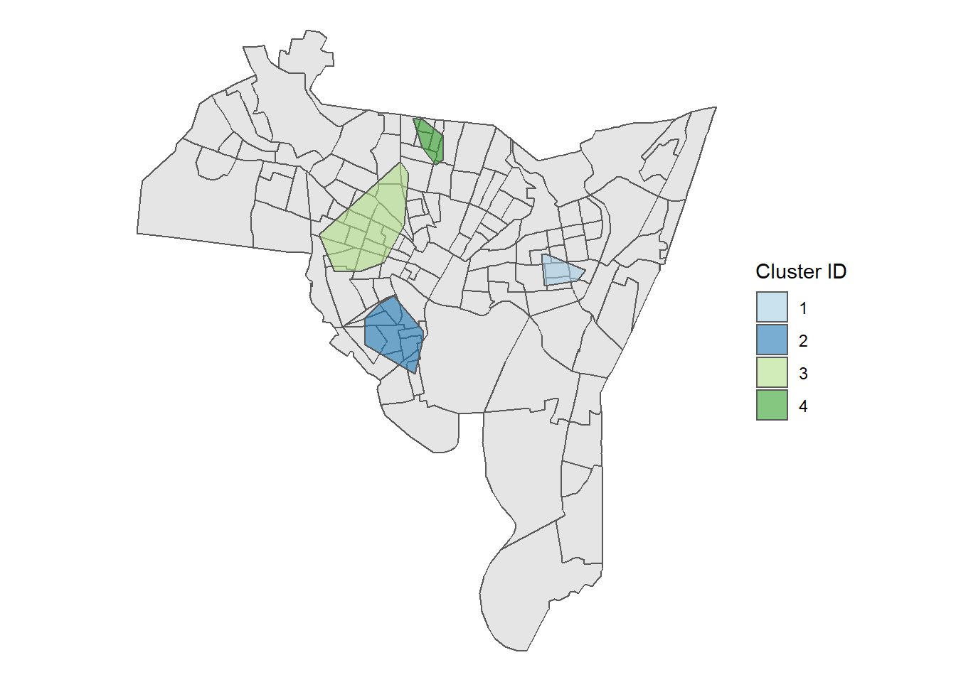
We can also add plot_points = TRUE to show the location of homicides on the map and print_area = TRUE to give
us some statistics about the size and scope of the clusters.
# Print out points

cluster_points(point_data = nh_homicides,
               polygon_data = nh_city,
               pts = 10,
               dist = 1500,
               plot_points = TRUE,
               print_area = TRUE)
## DBSCAN clustering for 161 objects.
## Parameters: eps = 1500, minPts = 10
## The clustering contains 4 cluster(s) and 66 noise points.
##
## 0 1 2 3 4
## 66 14 29 40 12
##
## Available fields: cluster, eps, minPts
## [1] "Proportion of Area: 4.11" "Proportion of Area: 1.94"
## [3] "Proportion of Area: 10.22" "Proportion of Area: 6.97"
## [5] "Proportion of Area: 6.64" "Proportion of Area: 4.76"
## [7] "Proportion of Area: 4.98" "Proportion of Area: 13.96"
## [9] "Proportion of Area: 27.42" "Proportion of Area: 21.85"
## [11] "Proportion of Area: 47.01" "Proportion of Area: 2.53"
## [13] "Proportion of Area: 34.13" "Proportion of Area: 12.63"
## [15] "Proportion of Area: 6.76" "Proportion of Area: 11.79"
## [17] "Proportion of Area: 40.32" "Proportion of Area: 26.62"
## [19] "Proportion of Area: 8.35" "Proportion of Area: 1.13"
## [21] "Proportion of Area: 5.71" "Proportion of Area: 10.89"
## [23] "Proportion of Area: 20.19" "Proportion of Area: 4.03"
## [25] "Proportion of Area: 21.18" "Proportion of Area: 14.02"
## [27] "Proportion of Area: 11.38" "Proportion of Area: 15.03"
## [29] "Proportion of Area: 11.6" "Proportion of Area: 11.48"
## [31] "Proportion of Area: 15.19" "Proportion of Area: 22.69"
## [33] "Proportion of Area: 12.24" "Proportion of Area: 21.6"
## [35] "Proportion of Area: 14.72" "Proportion of Area: 13.98"
## [37] "Proportion of Area: 23.11" "Proportion of Area: 12.92"
## [39] "Proportion of Area: 10.36" "Proportion of Area: 3.49"
## [41] "Proportion of Area: 19.11" "Proportion of Area: 10.93"
## [43] "Proportion of Area: 36.52" "Proportion of Area: 23.95"
## [45] "Proportion of Area: 19.21" "Proportion of Area: 27.45"
## [47] "Proportion of Area: 7.88" "Proportion of Area: 14.57"
## [49] "Proportion of Area: 16.59" "Proportion of Area: 23.11"
## [51] "Proportion of Area: 21.63" "Proportion of Area: 32.98"
## [53] "Proportion of Area: 37.66" "Proportion of Area: 14.99"
## [55] "Proportion of Area: 4.12" "Proportion of Area: 21.29"
## [57] "Proportion of Area: 19.52" "Proportion of Area: 19.02"
## [59] "Proportion of Area: 28.39" "Proportion of Area: 33.04"
## [61] "Proportion of Area: 32.57" "Proportion of Area: 14.18"
## [63] "Proportion of Area: 31.51" "Proportion of Area: 16.38"
## [65] "Proportion of Area: 32.86" "Proportion of Area: 54.87"
## [67] "Proportion of Area: 41.47" "Proportion of Area: 29.95"
## [69] "Proportion of Area: 31.67" "Proportion of Area: 34.09"
## [71] "Proportion of Area: 38.39" "Proportion of Area: 9.27"
## [73] "Proportion of Area: 14.79" "Proportion of Area: 27.12"
## [75] "Proportion of Area: 34.18" "Proportion of Area: 5.7"
## [77] "Proportion of Area: 19.56" "Proportion of Area: 51.15"
## [79] "Proportion of Area: 39.74" "Proportion of Area: 11.25"
## [81] "Proportion of Area: 13.09" "Proportion of Area: 37.03"
## [83] "Proportion of Area: 45.64" "Proportion of Area: 33.93"
## [85] "Proportion of Area: 18.69" "Proportion of Area: 14.99"
## [87] "Proportion of Area: 8.1" "Proportion of Area: 24.17"
## [89] "Proportion of Area: 19.44" "Proportion of Area: 9.12"
## [91] "Proportion of Area: 8.54" "Proportion of Area: 29.39"
## [93] "Proportion of Area: 69.12" "Proportion of Area: 15.48"
## [95] "Proportion of Area: 13.62" "Proportion of Area: 7.09"
## [97] "Proportion of Area: 19.75" "Proportion of Area: 121.99"
## [99] "Proportion of Area: 20.07" "Proportion of Area: 8.67"
## [101] "Proportion of Area: 33.75" "Proportion of Area: 5.52"
## [103] "Proportion of Area: 38.75" "Proportion of Area: 27.43"
## [105] "Proportion of Area: 21.13" "Proportion of Area: 15.26"
## [107] "Proportion of Area: 10.82" "Proportion of Area: 16.37"
## [109] "Proportion of Area: 26.8" "Proportion of Area: 1.14"
## [111] "Proportion of Area: 4.23" "Proportion of Area: 42.93"
## [113] "Proportion of Area: 24.83" "Proportion of Area: 5.79"
## [115] "Proportion of Area: 2" "Proportion of Area: 33.74"
## [117] "Proportion of Area: 19.43" "Proportion of Area: 11.82"
## [119] "Proportion of Area: 7.96" "Proportion of Area: 30.86"
## [121] "Proportion of Area: 8.75" "Proportion of Area: 25.37"
## [123] "Proportion of Area: 8.4" "Proportion of Area: 3.81"
## [125] "Proportion of Area: 1.17" "Proportion of Area: 6.13"
## [127] "Proportion of Area: 13.73" "Proportion of Area: 3.08"
## [129] "Proportion of Area: 1.22"
## [1] "Proportion of Incidents: 0.61"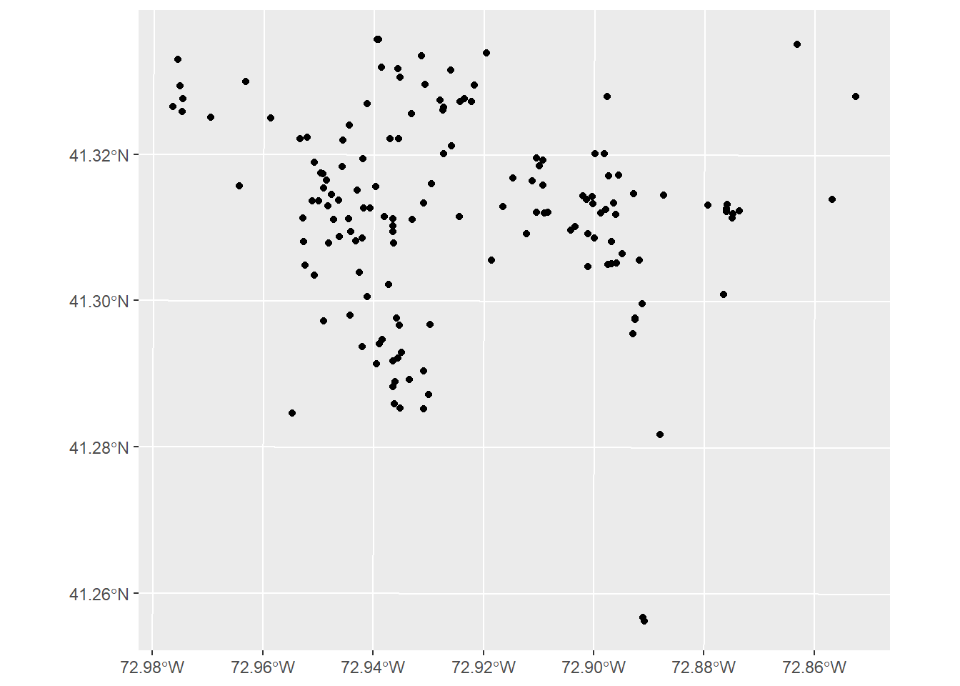
Now we see that our 4 clusters make up about 61% of all homicides in New Haven from 2010 through 2019. In terms of area, this is about 8% of New Haven in general. After identifying these clusters, we can then move on to the next step of analysis.