Chapter 9 Practice R

Statistical principles are used in most aspects of our daily lives; in choosing the lightest suitcase, the quietest street to live on, the biscuit with the most visible chocolate chips, the vaccine with a clinical trial that ticks the “most boxes”, the most commercially profitable business, and so on.

The way in which statistics is used and applied have be revolutionized over the past years. Machine learning techniques and sophisticated data science concepts/algorithms have expanded the scope for statistical applications.

The development of data science and machine learning concepts has also been accompanied by an advancement in the scope for data collection/capture. The availability of real time data capture, satellite images, and mobile apps has increased both the quantity and quality of data collection.

With sophisticated techniques for analysis and data collection there is a need for robust insight of core statistical concepts. Three early stages of statistical investigation are: construction of research hypotheses, data collection protocol, and data summarization/description.

Here, I begin with data summarization and focus on the measures of central tendency and measures of variation. I’ve used a fictional dataset, the chocolate biscuit dataset, to illustrate the concepts of central tendency and variation. This dataset is part of a “mystery series” which will be woven through the lectures so as to provide engaging applications to the statistical concepts presented.

In the Figure 1, I’ve used histograms to present a graphical overview of the number of chocolate chips found in bisucits within a chocolate biscuit factory before and after implementation of a policy. In the histograms for this example, the units on the x axis represent count categories of chocolate chips and the y axis represents the number of times (ie, the frequency) that a given count category is observed.

Simply put, Figure 1 illustrates the number of biscuits found with a given number of chocolate chips; before and after the new factory policy. Just for background, the policy requires that the employees refrain from eating inside the factory; this is because many biscuits have been discovered to be containing few chocolate chips and some biscuits seem to have been munched on.

In the histograms presented below, not only do we have a quick impression of the most frequently observed count of chocolate chips in biscuits (an indication of central tendency), but we also obtain an impression of the spread/distribution (an indication of variation) of the frequency of chocolate chip counts observed in the biscuits.

thebiscuits = read.csv("cookie_second_recipe.csv")
library(ggplot2)
library(kableExtra)
library(magrittr)
ggplot(thebiscuits, aes(x = chocolate_chips)) +
facet_wrap(. ~timeframe,ncol=1)+
geom_histogram(binwidth=1,aes(fill = ..count..)) +
scale_x_continuous(name = "Number of chocolate chips in biscuits ",breaks=c(1:30))  +
scale_y_continuous(name = "Count") +
ggtitle("Figure 1: Chocolate chips in biscuits at biscuit factory")+
theme(text = element_text(size=40))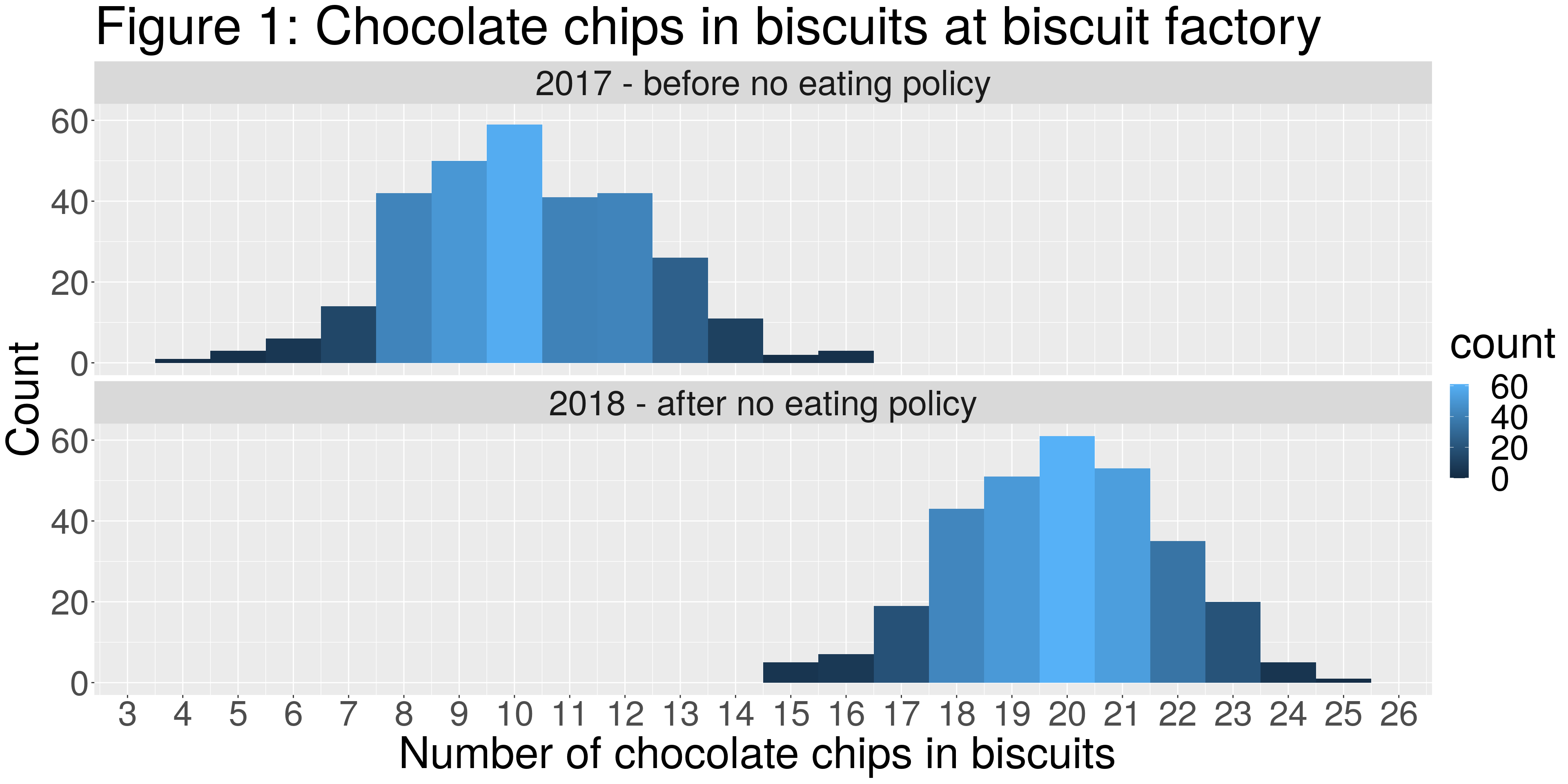

thebiscuits$chocolate_chips = round(thebiscuits$chocolate_chips,0)