2 Simple linear regression

The most elementary regression model is called the simple regression model, which is the model that we will use when only one x variable has an influence on the y variable. When we analyse the data, the process is called simple regression analysis. Usually, the first step in simple regression analysis is to construct a graph to express the relationship between the x and y variables. The simplest graph relating the variable y to a single independent variable x is a straight line. Thus we call the model a simple linear model or a simple straight-line model. Finally, the analysis of the data is then called simple linear regression analysis.

2.1 Scatter plots

The most effective way to display the relationship between two variables is to plot or graph the data. As we have mentioned before, this is usually the first step in simple linear regression analysis as this graph helps us to see at a glance the nature of the relationship to get a “feel” for what we are dealing with. The kind of graph we draw when we have two variables is called a scatter plot.

The scatter plot consists of a horizontal x-axis, a vertical y-axis and a dot for each pair of observations. Let’s have a look at an example that illustrates how to obtain a scatter plot

Example 2.1 It is often said that a person’s income is reflected in his or her savings. The more a person earns, the more he is likely to save. In this illustration the monthly income (x) will be the independent variable and savings (y) the dependent variable. In other words, we want to predict the savings by using monthly income as the predictor. The data for this example were collected for six randomly selected individuals and are given in the below.

Each data point or observation has two values: its x-value and its y-value and we call the two values a pair. Our sample of data in the table consists of 6 pairs of observations, which also indicates that the sample size, n, is equal to 6.

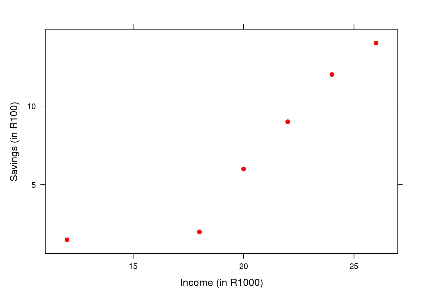
Figure 2.1: Scatter plot for income-savings data

2.2 Association between X and Y

2.3 The straight-line model

Why do we need the scatter plot? When a scatter plot displays a linear pattern, this pattern can be described by drawing a straight line through the dots. In practice, not all the dots will lie exactly on the line (we say that some dots deviate from the line) and the best line will be the one where these deviations are a minimum. These deviations are also called errors. Therefore we try to find a line that best fits the dots in the scatter plot, that is, a line that comes as close as possible to all the dots.

Why do we have to find this line? The answer is: in order to be able to make predictions. When the relationship between the x and y variables is strong, we will be able to predict fairly well, but when it is weak, our predictions will not be good at all.

What kind of predictions can we make? Predicting means saying what the y-value might be for a particular x-value. Let’s again have a look at the data given in Example 1. O nce we know the monthly income (x) of an individual, we can predict the savings of that individual (y). For example, if an individual has a monthly income of R23 000, how much is that individual going to save?

How do we find this best line in order to make predictions? We shall use a certain method to determine this line which is called the least squares method. The line is called the least squares regression line (or in short, the regression line) and working out this line is called simple linear regression analysis.

2.4 The simple linear model

The first step in determining the equation of the regression line that passes through the data points is to establish the equation’s form. In statistics, the form of the equation of the regression line is:

\[y = \beta_{0} + \beta_{1}*x + \epsilon\]

where:

y = Dependent variable

x = Independent variable

\(\beta_{0}\) = intercept, i.e. the point where the line touches or cuts through the y-axis when x equal 0.

\(\beta_{1}\) = slope, i.e. how much change in y-variable is caused by a unit change in x-variable.

\(\epsilon\) = random error component with \(\sim N(0, \sigma^{2})\)

The above equation is also called the first-order models, the straight-line model or simple linear regression model

When a relationship between the x and y variables exists, it means that the x-values have an influence on the y-values. Thus, if the x-values change, it will cause the y-values to also change. However, random error will occur because it is most likely that the changes in the x-values do not explain all the changes (or variability) that occur in the y-values. For example, suppose we want to predict the savings of an individual (y) through regression analysis by using the individual’s monthly income (x) as the predictor. Although savings are often related to income, there may be other factors that also have an influence on savings that are not accounted for by monthly income. Hence, a regression model to predict savings by only using the monthly income probably involves some error (the \(\epsilon\) that appears in the above equation). It is important to take these errors into account for all calculations in regression analysis.

The regression equation above can also be written as a regression line of means:

\[E(y) = \beta_{0} + \beta_{1}x\]

where E(y) = Expected value of y, i.e. the mean of the y-values. When the regression line of means is used, then \(\epsilon\) is equal to zero (the mean of the errors is equal to zero).

Our goal with these equations or models is to find values for \(\beta_{0}\) and \(\beta_{1}\) so that we can predict the y-value. However, virtually all regression analysis of business and other data involve sample data, not population data. As a result, \(\beta_{0}\) and \(\beta_{1}\) are unattainable and must be estimated by using sample data.

2.5 The least squares method

In order to select a regression line that provides the “best” estimate of the relationship between the independent and dependent variables, we will use the method of least squares. This method minimises the sum of the squares of the deviations (errors) of the observations from the regression line. The method of least squares provide us a sum of squared errors that is smaller than for any other straight-line model. The line obtained from this method is called the least squares line or regression line.

The equation for the regression line is also called the estimated regression model and \(\beta_{0}\) and \(\beta_{1}\) are called the regression coefficients. In order to use the regression line for predictions, we want to estimate the regression coefficients (determine their values by using the sample data). To estimate \(\beta_{0}\) and \(\beta_{1}\), we use the following steps and formulas:

1. Calculate \(\displaystyle\sum_{i=0}^{n}x_{i}\), \(\displaystyle\sum_{i=0}^{n} y_{i}\), \(\displaystyle\sum_{i=0}^{n} xy\), \(\displaystyle\sum_{i=0}^{n}x^{2}\), \(\bar{x}\), and \(\bar{y}\)

2. Calculate the sum of squares for \((SS_{xx}) = \displaystyle\sum_{i=0}^{n} x^{2} - n(\bar{x})^{2}\)

3. Calculate the sum of squares for \((SS_{xy}) = \displaystyle\sum_{i=0}^{n} xy - n(\bar{x})(\bar{y})\)

4. Calculate \(\hat{\beta_{1}} = \frac{SS_{xy}}{SS_{xx}}\)

5. Lastly calculate \(\hat{\beta_{0}} = \hat{y} - \hat{\beta_{1}}\bar{x}\)

After these coefficients are estimated, we write down the estimated regression model which we shall use for predictions.

Example 2.2 a) Fit the straight-line model to the income-savings data in Example 1. In order words, find the estimated values of the regression coefficients and write own the estimated model.

b) Plot the data points and graph the least squares line on the scatter plot.

Solution

a) Preliminary computations for the income-savings data are given below:

\(\displaystyle\sum_{i=0}^{n}x_{i} = 122, \qquad \displaystyle\sum_{i=0}^{n} y_{i} = 44.5, \qquad \displaystyle\sum_{i=0}^{n} xy = 1024, \qquad \displaystyle\sum_{i=0}^{n}x^{2} = 2604\),

\(\bar{x} = \frac{\displaystyle\sum_{i=0}^{n} x_{i}}{n} = 20.3333 \qquad \bar{y} = \frac{\displaystyle\sum_{i=0}^{n} y_{i}}{n} = 7.4167\)

\((SS_{xx}) = \displaystyle\sum_{i=0}^{n} x^{2} - n(\bar{x})^{2} = 2604 - 6(20.3333)^{2} = 2604 - 2480.6585 = 123.3415\)

\((SS_{xy}) = \displaystyle\sum_{i=0}^{n} xy - n(\bar{x})(\bar{y}) = 1024 - 6(20.3333)(7.4167) = 1024-904.8359 = 119.1641\)

\(\hat{\beta_{1}} = \frac{SS_{xy}}{SS_{xx}} = \frac{119.1641}{123.3415} = 0.9661\)

\(\hat{\beta_{0}} = \hat{y} - \hat{\beta_{1}}\bar{x} = 7.4167-0.9661(20.3333) = 7.4167 - 19.644 = -12.2273\)

Finally, we have to write down the estimated equation by replacing the \(\beta\) values by its estimated values:

\(\hat{y} = \hat{\beta_{0}} + \hat{\beta_{1}}x \implies \hat{y} = -12.2273 + 0.9661x\)

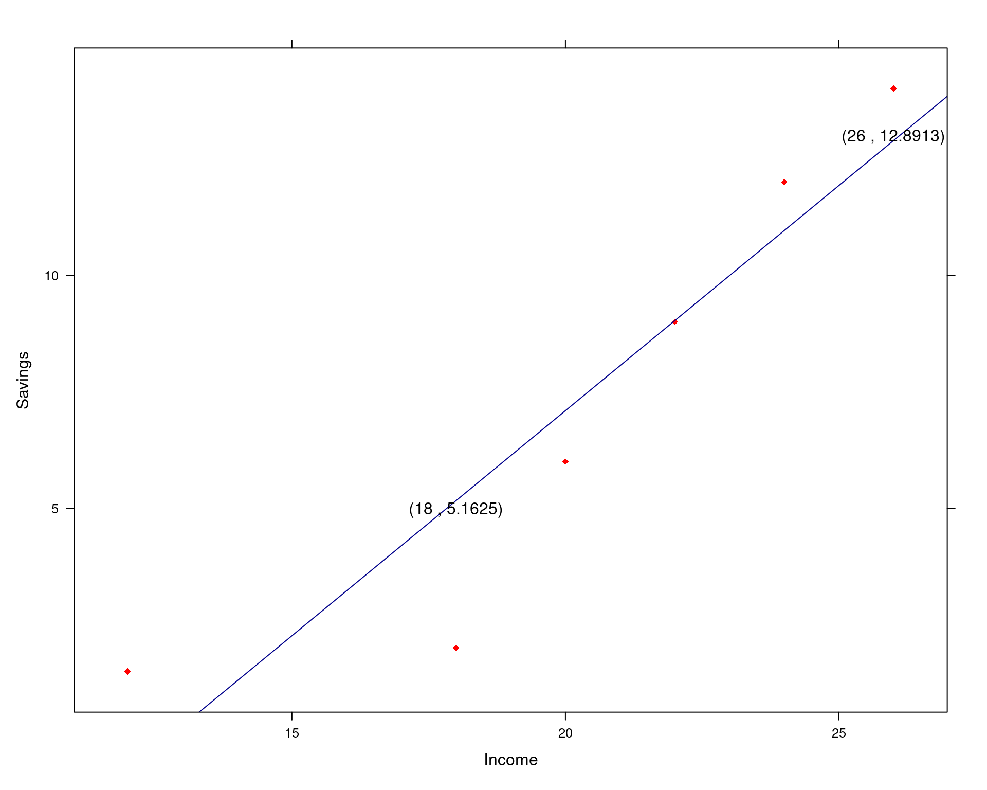
b) To plot the line on the scatter plot, we use the equation of the least squares line and determine the value of \(\hat{y}\) for two different values of x given in the sample data. We usually choose a smaller and a larger value; say we choose x = 18 and x = 26. Now we can determine \(\hat{y}\) for these two x-values:

for x = 18 \(\implies\) \(\hat{y} = -12.2273 + 0.9661(18) = -12.2273 + 17.3898 = 5.1625\)

for x = 26 \(\implies\) \(\hat{y} = -12.2273 + 0.9661(26) = -12.2273 + 25.1186 = 12.8913\)

Now we plot the two points (x , y) = (18 , 5.1625) and (26 , 12.8913) on the scatterplot and then draw a straight line through the two points. The regression line through the dots are given in the figure below.

2.5.1 How do I interpret the slope \(\hat{\beta_{1}}\) of the estimated regression model?

It is important that you be able to interpret the slope, \(\hat{\beta_{1}}\), in terms of the data being utilised to fit the model. If you calculate the value of the slope, the value actually means nothing. But if we interpret this value, it can tell us a “story” about the data. I.e., the interpretation helps to make sense of the data.

\(\color{red}{NB!!!}\) The interpretation of the value of $ \(\hat{\beta_{1}}\) is dependent on the sign (+ or -) of \(\hat{\beta_{1}}\). The meaning (interpretation) of the slope is about the following: If x changes with one unit, what will the expected change in y be?

The interpretation of \(\hat{\beta_{1}}\), is as follows:

If the value of \(\hat{\beta_{1}}\) is positive:

If x increases with one unit, then the average of y (or (E(Y)) ) will increase with \(\hat{\beta_{1}}\) units.

So, if the value of \(\hat{\beta_{1}}\) is positive, then the changes happen in the same direction.

If the value of \(\hat{\beta_{1}}\) is negative:

If x increases with one unit, then the average of y (or (E(Y)) ) will decrease with \(\hat{\beta_{1}}\) units.

So, if the value of \(\hat{\beta_{1}}\) is negative, then the changes happen in the opposite direction.

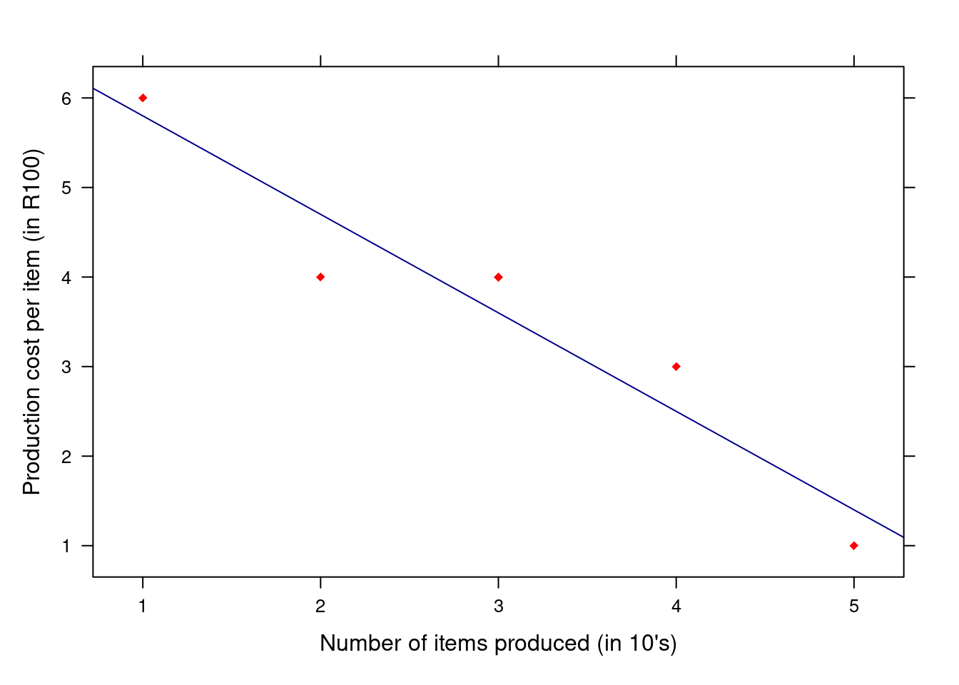
A company wants to investigate the relationship between the number of items produced, x (given in terms of 10 items), and the production cost per item, y (given in terms of R100). The data are given below.

\(x: \qquad 1 \quad 2 \quad 3 \quad 4 \quad 5\)

\(y: \qquad 6 \quad 4 \quad 4 \quad 3 \quad 1\)

1. Fit the straight-line model \(E(y) = \beta_{0} + \beta_{1}x\) to the data. In other words, estimate the values of \(\beta_{0}\) and \(\beta_{1}\) and write down the estimated equation.

2. Plot the data points and graph the least quares line on the scatter plot.

3. Interpret the value of the slope (\(\hat{\beta_{1}}\)).

Solution

\(\displaystyle\sum_{i=0}^{n}x_{i} = 15, \qquad \displaystyle\sum_{i=0}^{n} y_{i} = 18, \qquad \displaystyle\sum_{i=0}^{n} xy = 43, \qquad \displaystyle\sum_{i=0}^{n}x^{2} = 55\),

\(\bar{x} = \frac{\displaystyle\sum_{i=0}^{n} x_{i}}{n} = 3 \qquad \bar{y} = \frac{\displaystyle\sum_{i=0}^{n} y_{i}}{n} = 3.6\)

\((SS_{xx}) = \displaystyle\sum_{i=0}^{n} x^{2} - n(\bar{x})^{2} = 55 - 5(3)^{2} = 10\)

\((SS_{xy}) = \displaystyle\sum_{i=0}^{n} xy - n(\bar{x})(\bar{y}) = 43 - 5(3)(3.6) = -11\)

\(\hat{\beta_{1}} = \frac{SS_{xy}}{SS_{xx}} = \frac{-11}{10} = -1.1\)

\(\hat{\beta_{0}} = \hat{y} - \hat{\beta_{1}}\hat{x} = 3.6-(-1.1)(3) = 6.9\)

Finally, we have to write down the estimated equation by replacing the \(\beta\) values by its estimated values:

\(\hat{y} = \hat{\beta_{0}} + \hat{\beta_{1}}x \implies \hat{y} = 6.9 - 1.1x\)

b) To plot the line on the scatter plot, we use the equation of the least squares line and determine the value of \(\hat{y}\) for two different values of x given in the sample data. We usually choose a smaller and a larger value; say we choose x = 1 and x = 5. Now we can determine \(\hat{y}\) for these two x-values:

for x = 1 \(\implies\) \(\hat{y} = 6.9 - 1.1(1) = 5.8\)

for x = 26 \(\implies\) \(\hat{y} = 6.9 - 1.1(5) = 1.4\)

c) The value of \(\hat{\beta_{1}}\) is negative, then:

\(\implies\) If x increases with one unit, the average of y will decrease with 1.1 units and vice-versa

2.6 Using R to find the regression line

So why do you have to learn how to use and interpret computer printouts if the calculations discussed so far are so straightforward? Well, it is pretty obvious that, even with the use of a calculator, the process is laborious and susceptible to error. Fortunately, the use of statistical computer software can significantly reduce the labour involved in regression calculations. In addition, regression analysis typically involves working with large amounts of data. Since most practical regression problems are too large to be solved using hand calculations, you must be able to interpret the computer printouts (outputs) when statistical software are used to solve these problems.

Although many statistical software packages exist (SAS, SPSS, and MINITAB), you will learn how to use the outputs of the R packages. These statistical packages do lots of really cool things, but in this course you will learn about their capability of performing regression analysis. You’ll see that they are really great time savers!

When you look at the printouts, a lot of information is given. However, the first values that we are interested in are the estimated values of \(\beta_{0}\) and .\(\beta_{1}\).

Example 2.3 Using the lm function to obtain a simple linear model

To find the values of \(\beta_{0}\) and \(\beta_{1}\) lets look at the summary of the lm function. Is it possible observed thatwe have intercept and income. The (Intercept) represents \(\hat{\beta_{0}}\) and “income” represents \(\hat{\beta_{1}}\).

income <- c(24, 26, 12, 22, 20, 18)

savings <- c(12, 14, 1.5, 9, 6, 2)

model <- lm(savings ~ income)

summary(model)

## 
## Call:
## lm(formula = savings ~ income)
## 
## Residuals:
##        1        2        3        4        5        6 
##  1.04054  1.10811  2.13514 -0.02703 -1.09459 -3.16216 
## 
## Coefficients:
##             Estimate Std. Error t value Pr(>|t|)   
## (Intercept) -12.2297     3.9868  -3.068  0.03738 * 
## income        0.9662     0.1914   5.049  0.00724 **
## ---
## Signif. codes:  0 '***' 0.001 '**' 0.01 '*' 0.05 '.' 0.1 ' ' 1
## 
## Residual standard error: 2.125 on 4 degrees of freedom
## Multiple R-squared:  0.8644, Adjusted R-squared:  0.8305 
## F-statistic: 25.49 on 1 and 4 DF,  p-value: 0.007237

You see how easy it is! Without doing any calculations, you can instantly find the regression coefficients and just write down the estimated regression equation which is:

\[\hat{y} = -12.2297 + 0.9662x\]

2.7 The correlation coefficient (r) and the coefficient of determination \((R^{2})\)

2.7.1 The correlation coefficient (r) and its characteristics

Once the least squares line has been estimated, the significance (or strength) of the relationship must be evaluated. If there is a weak relationship between variables, there is no reason to use the estimated regression equation furthermore. Although a scatter plot can give us some information about the strength of the relationship, it will be useful to have a number that tells us exactly how strong or weak a relationship between the two variables is. In statistics, we call this number the Pearson product moment coefficient of correlation (in short, the correlation coefficient), and if it is calculated for the sample data, it is denoted by the symbol r.

So, how do we calculate the value of the correlation coefficient? You can use the following formula:

\[r = \frac{SS_{xy}}{\sqrt{SS_{xx}SS_{yy}}}\]

where:

\(SS_{yy} = \displaystyle\sum_{i=0}^{n} y^{2} - n(\bar{y})^{2}\)

\(SS_{xx} = \displaystyle\sum_{i=0}^{n} x^{2} - n(\bar{x})^{2}\)

\(SS_{xy} = \displaystyle\sum_{i=0}^{n} xy - n(\bar{x})(\bar{y})\)

Before we look at an example that illustrates how to calculate r, here are some facts about correlation that you need to know in order to interpret and make sense of the value of r.

• A correlation coefficient can only measure the strength of a linear relationship. It does not measure the strength of curved relationships, no matter how strong they are.
• The value of r is always between -1 and 1. A positive value indicates a positive relationship between the variables and a negative value indicates a negative relationship.
• r = -1 indicates a perfect negative linear correlation (which usually do not exists).
• r = 1 indicates a perfect positive linear correlation (which also usually do not exists).
• r = 0 indicates no linear correlation. It tells us that there is no linear relationship, but there might or might not be a non-linear relationship.
• According to the above, we can say that a value of r close to 0 implies little or no linear relationship between x and y. In contrast, the closer r is to -1 or 1, the stronger the linear relationship between x and y.
• Note that r is computed using the same quantities used in fitting the least squares line. Since both r and \(\beta_{1}\) provide information about the relationship between x and y, it is not surprising that there is a smilarity in their computational formulas. In particular, note that \(SS_{xy}\) appears in the enumarators of both expressions and, since denominators are always positive, r and \(\beta_{1}\) will always be of the same sign (either both positive or negative).

Example 2.4 Calculate the correlation coefficient for the income-savings data.

Solution

The quantities needed to calculate r are \(SS_{xx}\), \(SS_{xy}\) and \(SS_{yy}\). The first two quantities have been calculated previously and are repeated here for convenience. Let’s have a look at the data again.

\(\displaystyle\sum_{i=0}^{n}x_{i} = 122, \qquad \displaystyle\sum_{i=0}^{n} y_{i} = 44.5, \qquad \displaystyle\sum_{i=0}^{n} xy = 1024, \qquad \displaystyle\sum_{i=0}^{n}x^{2} = 2604\),

\(\bar{x} = \frac{\displaystyle\sum_{i=0}^{n} x_{i}}{n} = 20.3333 \qquad \bar{y} = \frac{\displaystyle\sum_{i=0}^{n} y_{i}}{n} = 7.4167\)

\((SS_{xx}) = \displaystyle\sum_{i=0}^{n} x^{2} - n(\bar{x})^{2} = 2604 - 6(20.3333)^{2} = 2604 - 2480.6585 = 123.3415\)

\((SS_{xy}) = \displaystyle\sum_{i=0}^{n} xy - n(\bar{x})(\bar{y}) = 1024 - 6(20.3333)(7.4167) = 1024-904.8359 = 119.1641\)

\((SS_{yy}) = \displaystyle\sum_{i=0}^{n} y^{2} - n(\bar{y})^{2} = 463.25 - 6(7.4167)^{2} = 463.25 - 330.0446 = 133.2054\)

\(r = \frac{SS_{xy}}{\sqrt{SS_{xx} ss_{yy}}} = \frac{119.1641}{\sqrt{123.3415 \times 133.2954}} = \frac{119.1641}{128.2219} = 0.9294\)

The correlation is very close to 1 which indicates that there is a very strong, positive correlation between “monthly income” and “savings”. This means that income(x) has a large influence on savings (y). The positive sign indicates that, if the monthly income (x) increases, the savings (y) will also increase or if the monthly income decreases, then the savings will also decrease.

2.7.2 Using R to calculate the coeffcient of correlation

income <- c(24, 26, 12, 22, 20, 18)

savings <- c(12, 14, 1.5, 9, 6, 2)

cor(income, savings)

## [1] 0.9297129

2.7.3 The coefficient of determination \((R^2)\)

The coefficient of determination is simply equal to r2. Note that \(R^{2}\) is always between 0 and 1. The closer the value of \(R^{2}\) is to 1, the better the line fits the data and the more accurate the predictions will be. The closer the value of \(R^{2}\) is to 0, the poorer the fit of the line and the less accurate the predictions will be. When calculating \(R^{2}\) , you can multiply your answer by 100 to get the percentage. So the closer \(R^{2}\) is to 100%, the greater the influence of x on y, the better the line fits the data and the more accurate the predictions will be.

So what does this value actually mean? It shows the proportion of variability (changes) of the dependent variable (y) accounted for or explained by the independent variable (x). Now this is a difficult definition, but let’s explain it in a simple way by looking at the income-savings data.

Example 2.5 Calculate the coefficient of determination for the income-savings data and interpret the value.

Solution

The value of r (0.9294) was already calculated. Therefore the value of the coefficient of determination, \(R^{2}\), is equal to \((0.9294)^{2}\) which is 0.8638. In percentage if \(0.8638 \times 100 = 86.38\%\).

This means that the changes (variation) in income (x) cause 86.38% of the changes (variation) in savings (y). This means that income is mainly responsible for the changes in savings. What about the remaining 13.62% of changes that happen in savings? We can say that other factors cause 13.62% of the changes in savings (y). It is clear that other factors do not have a large influence on savings and can be ignored. This is how we know that the changes in x (income) really cause the changes in y (savings). It also means that the linear model, was a good model to fit to the data and that the model can be used to predict the savings (y).

income <- c(24, 26, 12, 22, 20, 18)

savings <- c(12, 14, 1.5, 9, 6, 2)

cor(income, savings)^2 

## [1] 0.8643661

# 

model <- lm(savings ~ income)
summary(model)

## 
## Call:
## lm(formula = savings ~ income)
## 
## Residuals:
##        1        2        3        4        5        6 
##  1.04054  1.10811  2.13514 -0.02703 -1.09459 -3.16216 
## 
## Coefficients:
##             Estimate Std. Error t value Pr(>|t|)   
## (Intercept) -12.2297     3.9868  -3.068  0.03738 * 
## income        0.9662     0.1914   5.049  0.00724 **
## ---
## Signif. codes:  0 '***' 0.001 '**' 0.01 '*' 0.05 '.' 0.1 ' ' 1
## 
## Residual standard error: 2.125 on 4 degrees of freedom
## Multiple R-squared:  0.8644, Adjusted R-squared:  0.8305 
## F-statistic: 25.49 on 1 and 4 DF,  p-value: 0.007237

2.8 Model assumptions

For each observation in a sample of data, there is a random error \((\epsilon)\) involved. If our sample includes ten pairs of observations, then there are ten errors to account for. There are four basic assumptions about the error.

1. The mean of the probability distribution of \(\epsilon\) is 0. That is, the average of the errors over an infinitely long series of experiments is 0 for all values of x.

2. For each error, a variance exists. The variance of the probability distribution of \(\epsilon\) must be constant for all values of x. This means that the variances for all \(\epsilon\) are the same (or the variances are constant).

3. The probability distribution of \(\epsilon\) must be a normal distribution.

4. The errors associated with any two observations are independent. That is, the error associated with one observation has no effect on the errors associated with other observations.

These assumptions must be true in order for our regression results to be correct. For example, when these assumptions are not true, then our \(\beta_{0}\) and \(\beta_{1}\) values will be wrong and consequently our prediction of y will also be wrong. How do we know whether these assumptions are true or not? Various diagnostic techniques exist for checking the validity of these assumptions, which will be discussed in the second semester. So what happens if some or all of these assumptions are not true? Fortunately, there are remedies to be applied when the assumptions appear to be invalid. When applied, it will make the assumptions valid again and we can continue with our regression analysis process. These remedies will also be discussed in the second semester.

But for now, let’s assume that the assumptions are true or valid for each and every data set that we will use in this and future lectures. In the sections that follow, we will continue with the regression analysis process.

2.9 An estimator of the Random Error \((\epsilon)\)

In this section we will show you how to estimate this random error (i.e. how to find a value that will indicate the size of the error). It seems reasonable to assume that the greater the variability of the random error \((\epsilon_{i})\) the greater will be the errors in the estimation of the model parameters \(\beta_{0}\) and \(\beta_{1}\) and in the prediction of y for some values of x. For the population data, the random error is measured by its variance \(\sigma^{2}\) will be unknown. So how do we find a value for the random error? We use sample data to estimate \(\sigma^{2}\). For the sample data, the variance is denoted by \(S^{2}\).

Because we always have to take the random errors into account, you should not be surprised, as we proceed through this and other lectures, to find that \(S^{2}\) or s appears in almost all the formulas that we use. What is s? It is the square root of the variance \(S^{2}\) and we refer to it as the estimated standard error of the regression model, or in short, just the standard error or the standard deviation. To calculate the values of the sample variation and the standard error, the following formulas are used:

\[SSE = SS_{yy} - \hat{\beta_{1}} SS_{xy}\]

\[S^{2} = \frac{SSE}{n-2}\]

\[S = \sqrt{s^{2}}\]

where n is the number os the parameters in the regression model.

Example 2.6 Give an estimated valur for the standard error \((\epsilon)\) of the regression model for the income-savings data. Calculate the coefficient of variation and interpret the value. The following values were already calculated for the dara and are given here for convenience: \(SS_{yy} = 133.2054\), \(SS_{xy}=119.1641\), and \(\hat{\beta_{1}} = 0.9661\).

Solution

\(SSE = SS_{yy} - \hat{\beta_{1}} = 133.2054 - 0.9661(119.1641) = 133.2054-115.1244 = 18.081\)

\(S^{2} = \frac{SSE}{n-2} = \frac{18.081}{4} = 4.5203\)

\(S = \sqrt{S^{2}} = \sqrt{4.5203} = 2.1261\)

Now you know how to calculate the values of \(S^{2}\) and S. However, the values of \(S^{2}2\) and S can also be obtained from a simple linear regression printout. We must remember that the variance is also called the Mean Square Error (MSE). So this is the name that we have to look out for if we want to find the variance. In the R printout, the value of the standard error S is denoted by Residual standard error.

income <- c(24, 26, 12, 22, 20, 18)

savings <- c(12, 14, 1.5, 9, 6, 2)

model <- lm(savings ~ income)
summary(model)

## 
## Call:
## lm(formula = savings ~ income)
## 
## Residuals:
##        1        2        3        4        5        6 
##  1.04054  1.10811  2.13514 -0.02703 -1.09459 -3.16216 
## 
## Coefficients:
##             Estimate Std. Error t value Pr(>|t|)   
## (Intercept) -12.2297     3.9868  -3.068  0.03738 * 
## income        0.9662     0.1914   5.049  0.00724 **
## ---
## Signif. codes:  0 '***' 0.001 '**' 0.01 '*' 0.05 '.' 0.1 ' ' 1
## 
## Residual standard error: 2.125 on 4 degrees of freedom
## Multiple R-squared:  0.8644, Adjusted R-squared:  0.8305 
## F-statistic: 25.49 on 1 and 4 DF,  p-value: 0.007237

2.10 Inference about the slope

Conducting a hypothesis test for the slope \((\hat{\beta_{1}})\) is important to see if the population slope \((\beta_{1})\) is significantly different from zero. If the population slope is not different from zero, we can conclude that the sample regression model has no predictability of the dependent variable y, and the model therefore has little or no use.

How do we conduct this hypothesis test to get more information about the slope of the population? We start by specifying the null and alternative hypotheses:

\[H_{0}: \beta_{1} = 0\]

\[H_{1}: \beta_{1} \neq 0 \qquad \text{or} \qquad \beta_{1} > 0 \qquad \text{or} \qquad \beta_{1} > 0\]

If it the null hypothesis could talk, it would say something like “I represent no linear relationship between the variables of the population that you are studying”. The alternative hypothesis is equally interesting. If it could talk, it would say something like “I represent a relationship between the variables of the population, or, I represent a positive or a negative relationship between the variables of the population”. Remember that the null and alternative hypotheses always refer to the population and are always written using Greek symbols.

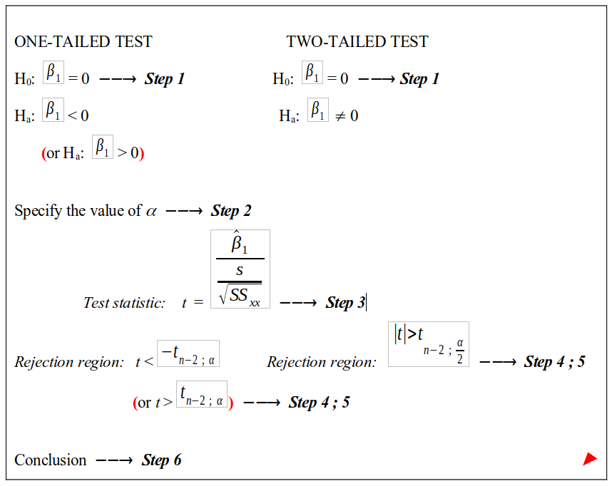
2.11 The t-test for the slope

To determine whether a significant linear relationship between the population variable x and y exists, we will perform a hypothesis test which we call a t-test. We usually follow six steps to perform a hypothesis test:

1. State the null and alternative hypothesis. Remember that the null hypothesis is always equal to (=) a certain vale and that the alternative hypothesis can be larger than (>), smaller than (<) or not equal to \((\neq)\) that same value. In this case the value is zero.

2. State the value of \(\alpha\)

3. Determine the test statistic. This test statistic is actually a formula that we use to calculate a certain value.

4. Determine the critical value.

5. Decide to reject \(H_{0}\) or not to reject \(H_{0}\) by using the rejection rules.

6. Given a conclusion

The figure below shows how to find the information needed in the different steps.

Example 2.7 It is generally accepted that interest rates provide an excellent leading indicator for predicting the number of building projects that commences during a given year. As interest rates change the number of building projects that commence also seem to change. A market researcher decides to study this possible relationship and collects the following data on the prevailing interest rate and the recorded number of building permits issued in a certain region over a 12-year period:

The following values are known. (Determine these values on your own as an extra exercise)

\(SS_{xx} = 53.25\) \(SS_{xy}=-1670.5\) \(SS_{yy} = 59296\)

\(\hat{\beta_{1}}=-31.3709\) \(SSE = 6890.9249\) \(S=26.2506\)

We want to know if a negative linear relationship exists between interest rate and the annual number of building permits issued. Test at a 5% level of significance. The performance of the hypothesis test will now be discussed step-by-step.

Solution

1. State \(H_{0}\) and \(H_{a}\). We have to go back to the question to decide what sign will be used in \(H_{a}\). The question ask us to test for negative linear relationship and therefore the sign is “<”. The answers for step 1 is :

\(H_{0}: \beta_{1} = 0\)

\(H_{a}: \beta_{1} < 0\)

2. When testing at 5% levels of significance, so \(\alpha = 5\%\)

3. Determine the test statistic by using the formula

\(t_{calc} = \frac{\frac{\hat{\beta_{1}}}{S}}{\sqrt{SS_{xx}}} \quad = \quad \frac{\frac{-31.3709}{26.2506}}{\sqrt{53.25}} \quad = \quad \frac{-31.3709}{3.5973} \quad = \quad -8.7207\)

4. The critical value depend on the level of significance. The critical value given by the rejection region is:

\[t_{n-2; \alpha} = t_{10; 0.05}\]

Now we have to get this value from the t-distribution table. Find the first value, namely 10, in the very first column of the table. Go down the column until you reach the value 10. Find the second value, namely 0.05, in the very first row of the table. That is, go to \(t_{.050}\) in the first row. The intersection of \(t_{.050}\) and the value 10 gives the critical value we need. Therefore

\(t_{(10;\alpha)} = -1.812\), where -1.812 is the critical value.

The critical value depends on the sign used in the alternative hypothesis. Because the sign is “V”, we have a one-tailed test and we go to the rejection region on the left hand side of the box.

Using R to find the critical value

qt(p, df), where p is the probability of error \((\alpha)\) and df is n-2

qt(0.05, 10)

## [1] -1.812461

5. What does the rejection region of the one-tailed test tells us? The rejection region is given as \(t_{calc} < t_{(n-2;\alpha)}\) and it means that we reject \(H_{0}\) if the value of \(t_{calc}\) is smaller than the \(t_{(n-2;\alpha)}\). Now lets see: \(t_{calc} = -8.7207\), and \(t_{tab}=-1.812\). Therefore \(t_{calc}\) is smaller than \(t_{tab}\), so we reject \(H_{0}\).

6. Conclusion: We reject \(H_{0}\), so \(\hat{\beta_{1}}\) is smaller than 0. This means that, if the interest rate increases, the number of building permits decreases.

2.11.1 R output

interest <- c(16.5,16,16.5,17.5,18.5,19.5,20,19,17.5,19,21.5,23.5)

build <- c(217,294,278,194,175,154,96,131,205,170,86,52)


model <- lm(build ~ interest)

summary(model)

## 
## Call:
## lm(formula = build ~ interest)
## 
## Residuals:
##     Min      1Q  Median      3Q     Max 
## -35.786 -18.306  -1.286  12.635  36.730 
## 
## Coefficients:
##             Estimate Std. Error t value Pr(>|t|)    
## (Intercept)  759.204     67.874  11.185 5.64e-07 ***
## interest     -31.371      3.597  -8.721 5.49e-06 ***
## ---
## Signif. codes:  0 '***' 0.001 '**' 0.01 '*' 0.05 '.' 0.1 ' ' 1
## 
## Residual standard error: 26.25 on 10 degrees of freedom
## Multiple R-squared:  0.8838, Adjusted R-squared:  0.8722 
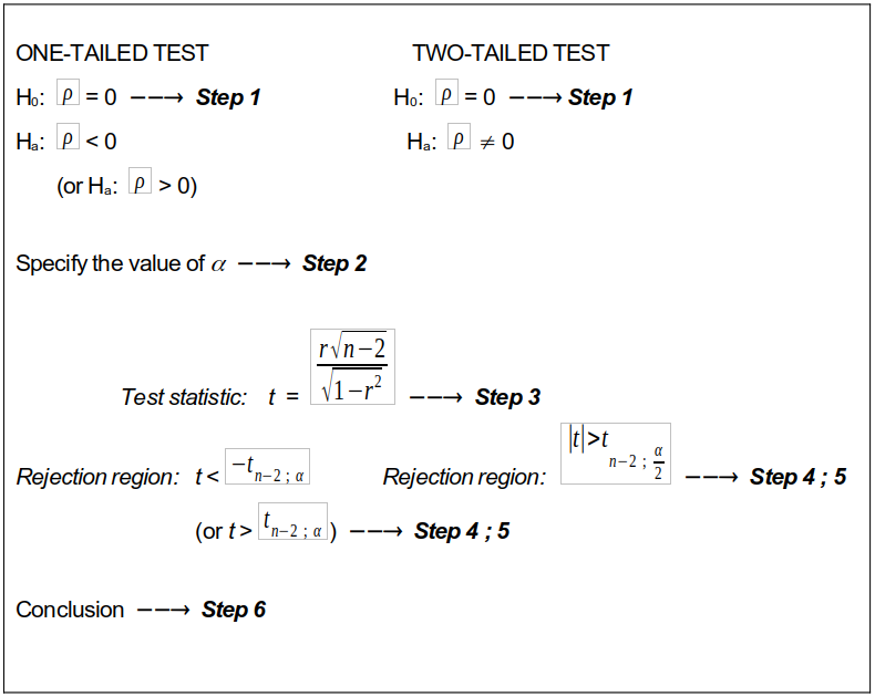
## F-statistic: 76.05 on 1 and 10 DF,  p-value: 5.489e-06

2.12 Hypothesis test for correlation (r)

The previous hypothesis tests were performed to statistically determine whether a linear relationship or regression exists between the variables. In this section we will discuss another hypothesis test which is about determining whether a correlation between the variables exists. Keep in mind that the correlation coefficient r measures the correlation (strength) between x-values and y-values for the sample data. But, a similar coefficient of correlation exists for the whole population of data from which the sample was selected. So, we want to know whether there is any evidence of a statistically significant correlation between the x-values and the y-values of the population of data. By now you know that, if we want more information about the population of data, we have to perform a hypothesis test. If r denotes the correlation for the sample data, what symbol are we going to use to denote the population correlation coefficient? The population correlation coefficient is denoted by the symbol \((\rho)\). The procedure to test for correlation between two variables is outlined in the figure below.

Example 2.8 Test at a 5% level of significance whether a linear correlation exists for the income-savings data. Recall that r was previously calculated as 0.9294 and \(R^{2}\) as 0.8638.

Solution

1. Hypothesis

\(H_{0}: \rho = 0\)

\(H_{a}: \rho \neq 0\)

2. \(\alpha = 5\%\)

3. \(t_{calc} = \frac{r\sqrt{n-2}}{\sqrt{1-r^{2}}}\) = \(\frac{0.9294\sqrt{6-2}}{\sqrt{1-0.8638}}\) = \(\frac{1.8588}{0.3691}\) = 5.036

4. \(t_{tab} {(n-2; \quad \frac{\alpha}{2})}\) = \(t_{tab}(6-2; \quad \frac{0.05}{2})\) = \(t_{tab}(4;0.025)\) = 2.776

5. Reject \(H_{0}\) if \(|t_{calc}| > t_{tab}\)

6. Conclusion

Reject \(H_{0}\). There is a significant linear correlation between the population monthly income and savings at the 5% level of significance.

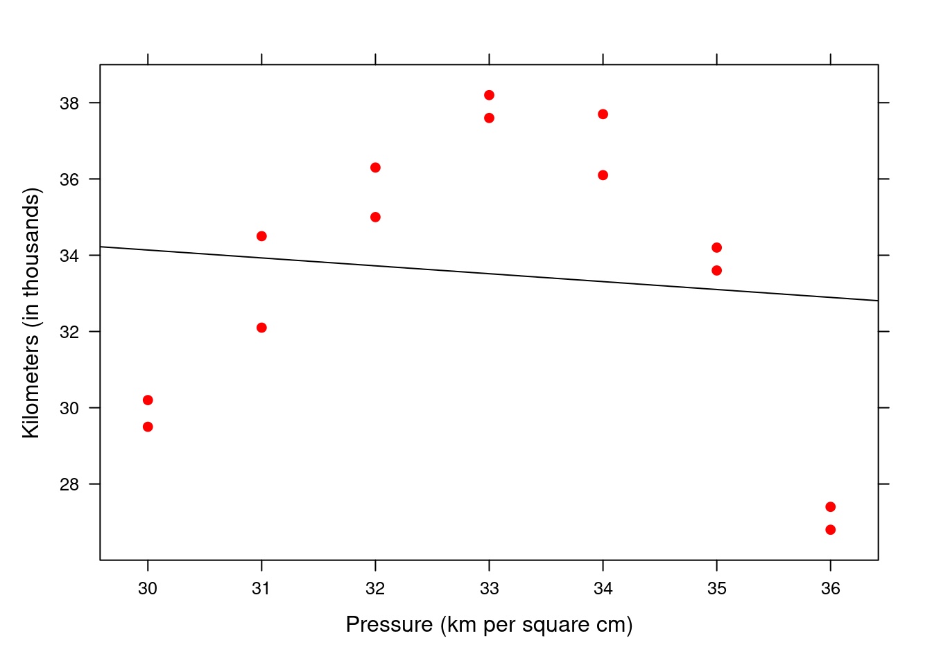
Example 2.9 Underinflated or overinflated tires can increase tire wear and fuel usage. A manufacturer of a new tire tested the tire for wear at different pressures. The correlation coefficient r was calculated as 0.1138. The dataset is below.

1. Interpret the value of r.

2. Determine the value of the coefficient of determination and interpret the value.

3. Test at a 10% level of significance whether a linear correlation between pressure and number of kilometers before the tire is weared out exists.

4. According to the above results, do you think we should continue with our regression analysis and why/why not?

Solution

1. The value of r is very close to zero and therefore there is a very weak, negative linear correlation between pressure and number of kilometers.

2. \(R^{2} = 0.013\) = 1.3%. Pressure has a weak influence on wear. Other factors cause 98.7% of the changes in wear and should also be taken into account. The pressure (x) is definitely not the main cause of the changes in y.

1. Hypothesis

\(H_{0}: \rho = 0\)

\(H_{a}: \rho \neq 0\)

2. \(\alpha = 10\%\)

3. \(t_{calc} = \frac{r\sqrt{n-2}}{\sqrt{1-r^{2}}}\) = \(\frac{-0.1138\sqrt{14-2}}{\sqrt{1-(-0.1138)^{2}}}\) = \(\frac{-0.3942}{0.9935}\) = -0.3938

4. \(t_{tab} {(n-2; \quad \frac{\alpha}{2})}\) = \(t_{tab}(14-2; \quad \frac{0.10}{2})\) = \(t_{tab}(12;0.05)\) = 1.782

5. Reject \(H_{0}\) if \(|t_{calc}| > t_{tab}\)

6. Conclusion

Don’t reject \(H_{0}\). There is no significant linear correlation between the tire pressure and wear at the 10% of error.

4. All the results above indicate that there is a weak linear correlation between pressure and number of kilometres. So, we should not continue with the linear regression analysis process.

2.12.1 Using R for the correlation test of significance

pressure <- c(30,30,31,31,32,32,33,33,34,34,35,35,36,36)

km <- c(29.5,30.2,32.1,34.5,36.3,35.0,38.2,37.6,37.7,36.1,33.6,34.2,26.8,27.4)

cor.test(pressure, km, conf.level=0.90)

## 
##  Pearson's product-moment correlation
## 
## data:  pressure and km
## t = -0.39647, df = 12, p-value = 0.6987
## alternative hypothesis: true correlation is not equal to 0
## 90 percent confidence interval:
##  -0.5442297  0.3642162
## sample estimates:
##        cor 
## -0.1137098

xyplot(km ~ pressure, xlab="Pressure (km per square cm)", ylab="Kilometers (in thousands)", pch=19, col="red",
       panel=function(x, y,...){
             panel.xyplot(x, y, ...)
             panel.lmline(x, y, col.line="black")
             }
             )