6 A quadratic (second-order) model with a quantitative predictor
The previous multiple regression models discussed so far (the first-order model and the interaction model), proposed straight-line relationships. However, if you look at some scattergrams of data sets, the scattergram is in the form of a curve. When this happens, we cannot use the previous two models, because they represent straight-line relationships between the x variables and y). Thus, to compensate for the curves present in the data, we have to fit a quadratic or second-order model to the data.
We shall start with a very simple quadratic model where there is only one x variable that have an influence on y. Now, when this is the case, we usually fit the straight-line model \(E(y) = \beta_{0} + \beta_{1}x\) to the data, as the scatterplots indicate straight lines. But, if the scatterplots indicates a curve, we can no longer use this model.
So, when curves occur in the scattergrams, then we know that the quadratic model must be fitted to the data. The model looks like this:
\[E(y) = \beta_{0} + \beta_{1}x + \beta_{2}x^{2}\]
We include the x variable in the model as usual, but then add the term \(\beta_{2} x^{2}\) which is called the quadratic term or the second-order term. This term represents the curvature in the data.
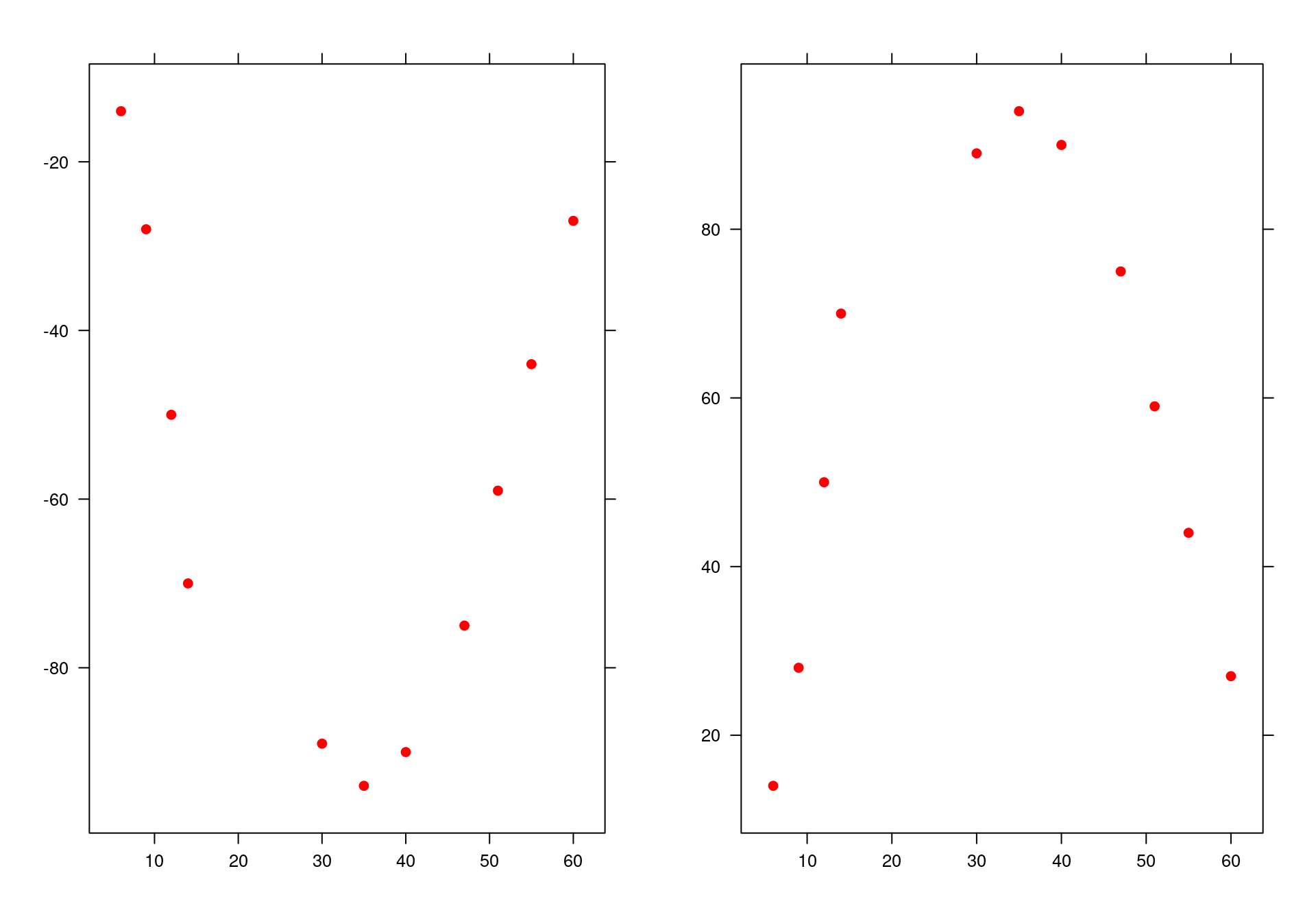
There are two types of curves when we have only one x variable that have an influence on y (see graphs above). The curve on the left-hand side is called a concave upward curvature, whilst the curve on the right is called a concave downward curvature. When we have a concave upward curvature (curve on the left), the value of \(\beta_{2}\) in the second-order model given above is positive (> 0) and when we have a concave downward curvature (curve on the right), the value of \(\beta_{2}\) is negative (< 0). Remember this for short questions.
Now lets have a look at an example to see what type of questions can be expected when we fit the quadratic model to a data set when one x variable have an influence on y. As I said before, the tests and interpretations are the same as we are used to by now, but we only have a different model to deal with.
Example 6.1 This example is about a person’s immune system and the effect of exercise on the immune system. They measure the immune system by the amount of immunoglobulin (I’m not a doctor, so don’t know what this is) in a blood sample. We call it IgG in short. They believe that the amount of IgG is related to the maximum oxygen uptake when you do exercise. The more oxygen you get, the better your immune system (and the higher IgG in the blood). The data set is given below – the data for IgG (y) and maximum oxygen uptake (x). So we have only one quantitative x variable that have an influence on y. If we go to the scattergram, given below the data set, you can see that it is in the form of a curve and not a straight line.
After fitting the quadratic model to the data, the results are given in the R printout provided. Now lets have a look at the questions related to this example.
Use the method of least squares to estimate the unknown beta parameters in the quadratic model.
Test at a 1% level of significance whether the overall model (that is the quadratic model) is useful for predicting the IgG. Use a critical value to perform the test.
Interpret the adjusted coefficient of determination
Predict the immunity (IgG) when the maximum oxygen uptake is 53 milliliters per kilogram.
Solution
igg <- c(881, 1290, 2147, 1909, 1282, 1530, 2067, 1982, 1019, 1651, 752, 1687, 1782, 1529, 969, 1660,2121,1382,1714,1959,1159,965,1456,1273,1418,1743,1997,2177,1965,1264)

oxygen <- c(34.6,45,62.3,58.9,42.5,44.3,67.9,58.5,35.6,49.6,33,52,61.4,50.2,34.1,52.5,69.9,38.8,50.6,69.4,37.4,35.1,43,44.1,49.8,54.4,68.5,69.5,63,43.2)library(lattice)
xyplot(igg ~ oxygen, pch=19, col="red")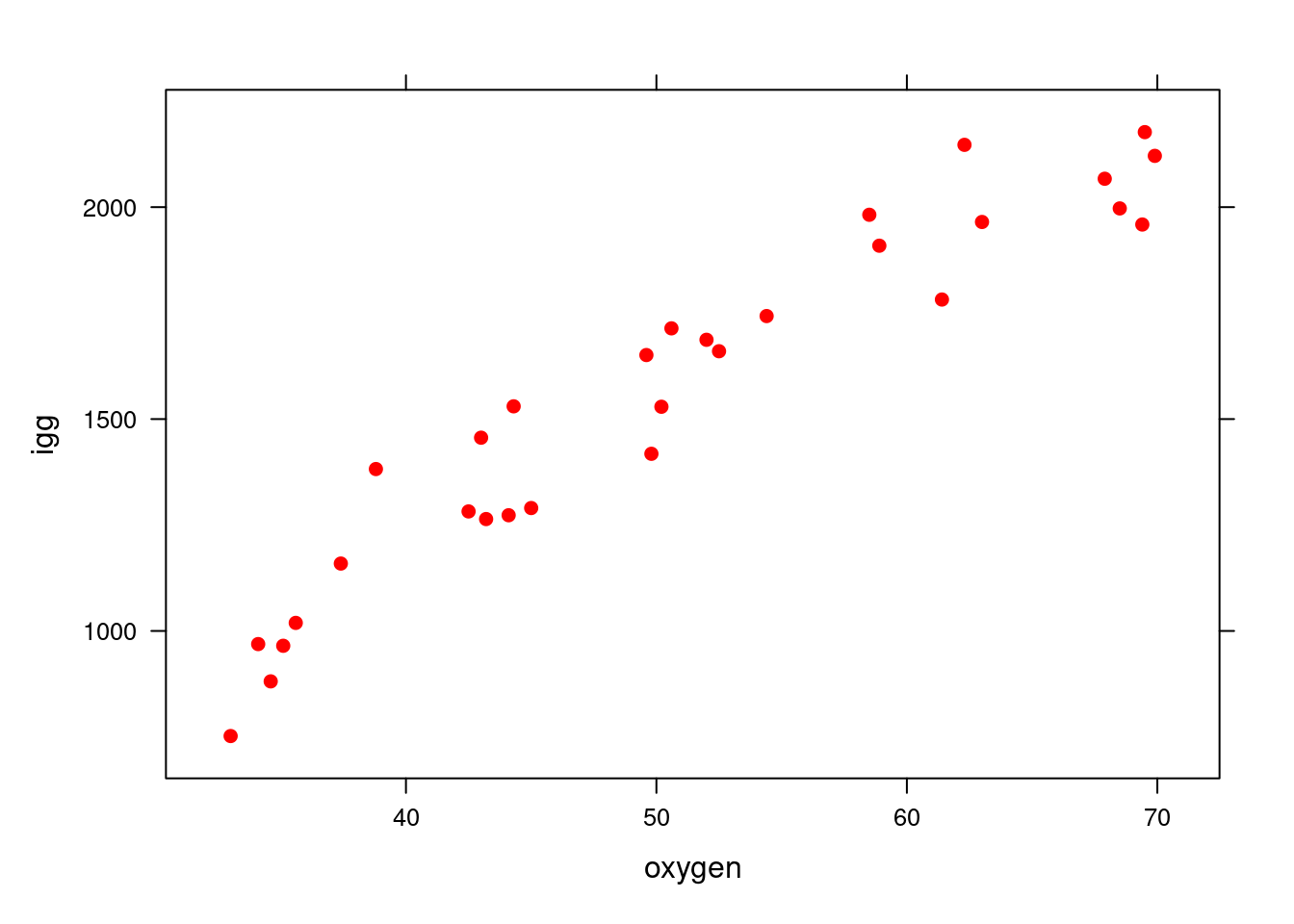
Quadratic model
model <- lm(igg ~ oxygen + I(oxygen^2))

anova(model)
## Analysis of Variance Table
##
## Response: igg
## Df Sum Sq Mean Sq F value Pr(>F)
## oxygen 1 4471180 4471180 394.57 < 2.2e-16 ***
## I(oxygen^2) 1 130091 130091 11.48 0.002175 **
## Residuals 27 305959 11332
## ---
## Signif. codes: 0 '***' 0.001 '**' 0.01 '*' 0.05 '.' 0.1 ' ' 1summary(model)##
## Call:
## lm(formula = igg ~ oxygen + I(oxygen^2))
##
## Residuals:
## Min 1Q Median 3Q Max
## -185.390 -82.163 1.053 66.688 227.302
##
## Coefficients:
## Estimate Std. Error t value Pr(>|t|)
## (Intercept) -1463.8326 411.4957 -3.557 0.00141 **
## oxygen 88.2885 16.4773 5.358 1.16e-05 ***
## I(oxygen^2) -0.5361 0.1582 -3.388 0.00217 **
## ---
## Signif. codes: 0 '***' 0.001 '**' 0.01 '*' 0.05 '.' 0.1 ' ' 1
##
## Residual standard error: 106.5 on 27 degrees of freedom
## Multiple R-squared: 0.9377, Adjusted R-squared: 0.933
## F-statistic: 203 on 2 and 27 DF, p-value: < 2.2e-16Quadratic model: \(E(y) = -1463.8326 + 88.2885x - 0.5361 x^{2}\)
The analysis of variance indicated that the coefficients for \(\beta_{1}\) and \(\beta_{2}\) are different of 0 at 5% probability of error. Therefore, there is evidence that the quadratic model fits the data.
Hypothesis
\(H_{0}: \beta_{i} = 0\)
\(H_{a}: \beta_{i} \neq o\)
After adjusting for the sample size and number of beta parameters in the model, the second-order model explain 93.3% of the changes in IgG (y). The model has a large influence on y and is therefore a good model to fit to the data.
\(y = -1463.8326 + 88.2885x - 0.5361 x^{2} \quad -1463.8326 + 88.2885(53) - 0.5361 (53)^{2} = \quad 1709.553\)
library(latticeExtra)##
## Attaching package: 'latticeExtra'## The following object is masked from 'package:ggplot2':
##
## layerpred <- predict(model)
xyplot(igg ~ oxygen, pch=19, col="red", xlab="Maximum Oxygen Uptake (milimeters per kilogram)", ylab="IgG (miligrams)") +
as.layer(xyplot(pred ~ oxygen, type="a", col="blue"))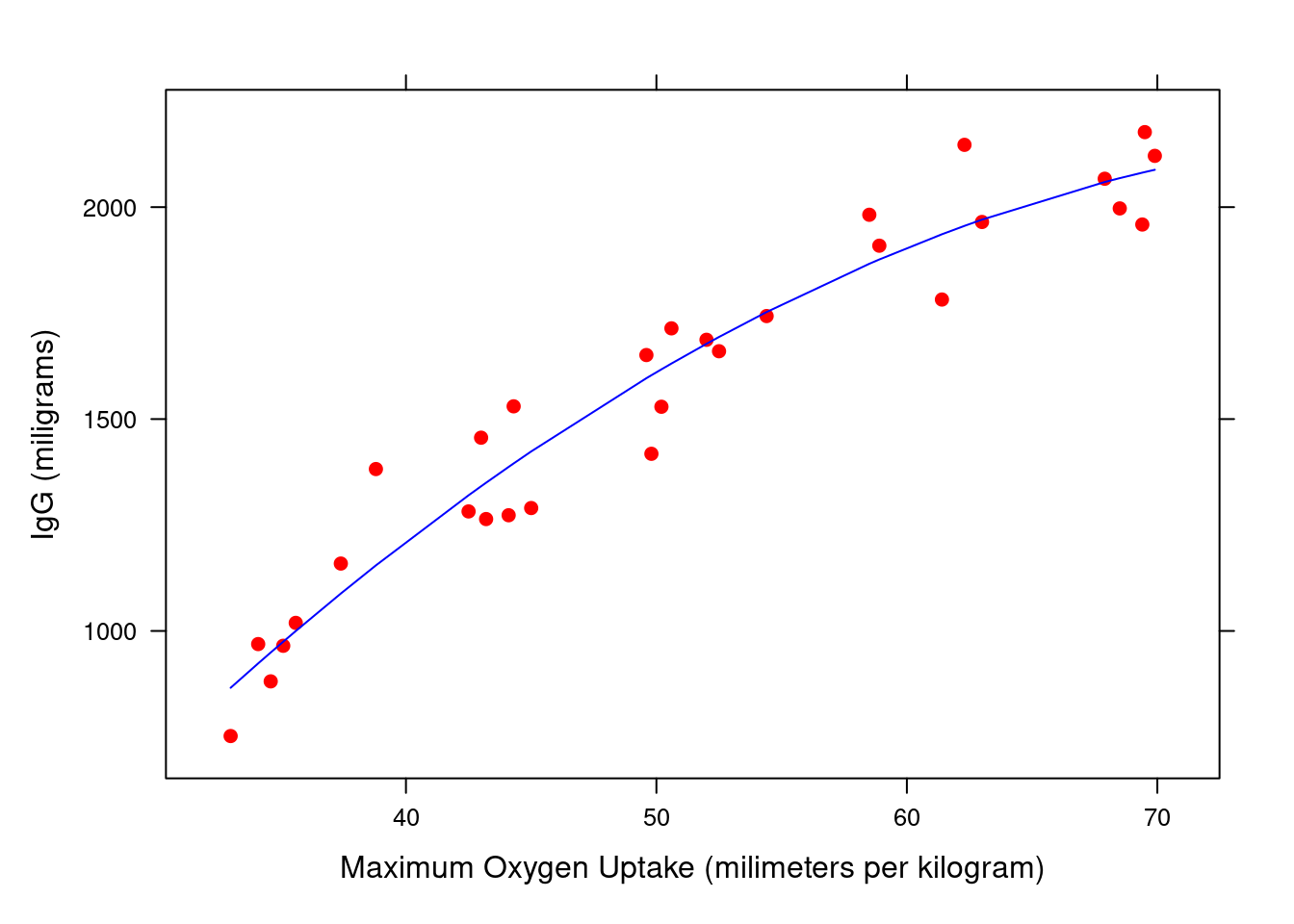
Interpretation of the \(\beta\) values
It only make sense to interpret the beta values when we have straight lines. However, it does not make sense to interpret the estimated beta values when a curve is present. The only conclusion that we can make from the beta values is to look at the sign of the value of \(\beta_{2}\) = -0.536. The sign is negative, and we can conclude that the curvature is concave downward. On the other hand, if the value of \(\beta_{2}\) is positive, then we conclude that the curve is concave upward. So this is the only information that can be extracted when we look at the beta values.