5 An interaction model with quantitative predictors
When two or more independent variables are involved in research, there is more to consider than just the ‘main effect’ of each of the independent variables (also called ‘factors’). This means that the effect of one independent variable on the dependent variable of interest may not be the same at all levels of the other independent variable. Another way of saying this is that the effect of one independent variable may depend on the level of the other independent variable.
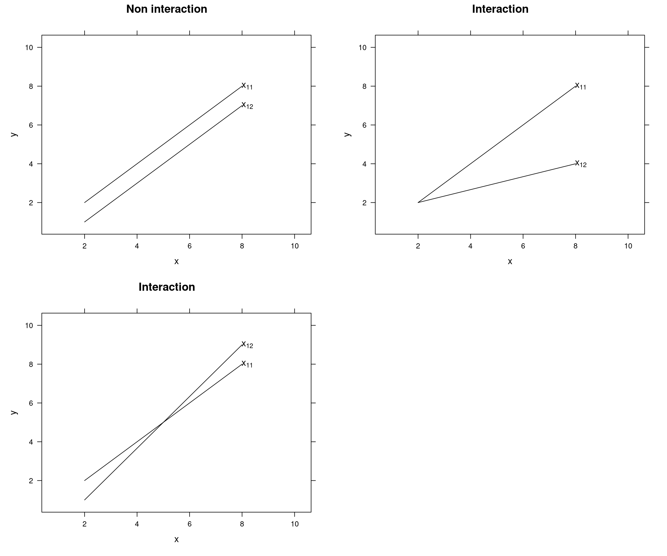
Figure 5.1: Non interaction and interaction examples
When the x’s are dependent, we say that \(x_{1}\) and \(x_{2}\) interact. Therefore we have to add an interaction term to the simple first-order model and then the model is called an interaction model. The interaction term is just the multiplication of the two x variables. The model is
\[E(y) = \beta_{0} + \beta_{1} x_{1} + \beta_{2} x_{2} + \beta_{3} x_{1} x_{2}\]
The term \(\beta_{3} x_{1} x_{2}\) is called the interaction term.
We will have situations when more than two x variables have an influence on y. Below is an example of what the interaction models look like if this is the case.
\[E(y) = \beta_{0} + \beta_{1} x_{1} + \beta_{2} x_{2} + \beta_{3} x_{3} + \beta_{4} x_{1} x_{2} + \beta_{5} x_{1} x_{3} + \beta_{6} x_{2} x_{3}\]
Example 5.1 We’ll use the marketing data set to predict sales units on the basis of the amount of money spent in the three advertising medias (youtube, facebook and newspaper)
library(datarium)

data(marketing)

head(marketing)
## youtube facebook newspaper sales
## 1 276.12 45.36 83.04 26.52
## 2 53.40 47.16 54.12 12.48
## 3 20.64 55.08 83.16 11.16
## 4 181.80 49.56 70.20 22.20
## 5 216.96 12.96 70.08 15.48
## 6 10.44 58.68 90.00 8.64First-order model
m1 <- lm(sales ~ youtube + facebook + newspaper, data=marketing)

anova(m1)
## Analysis of Variance Table
##
## Response: sales
## Df Sum Sq Mean Sq F value Pr(>F)
## youtube 1 4773.1 4773.1 1166.7308 <2e-16 ***
## facebook 1 2225.7 2225.7 544.0501 <2e-16 ***
## newspaper 1 0.1 0.1 0.0312 0.8599
## Residuals 196 801.8 4.1
## ---
## Signif. codes: 0 '***' 0.001 '**' 0.01 '*' 0.05 '.' 0.1 ' ' 1summary(m1)##
## Call:
## lm(formula = sales ~ youtube + facebook + newspaper, data = marketing)
##
## Residuals:
## Min 1Q Median 3Q Max
## -10.5932 -1.0690 0.2902 1.4272 3.3951
##
## Coefficients:
## Estimate Std. Error t value Pr(>|t|)
## (Intercept) 3.526667 0.374290 9.422 <2e-16 ***
## youtube 0.045765 0.001395 32.809 <2e-16 ***
## facebook 0.188530 0.008611 21.893 <2e-16 ***
## newspaper -0.001037 0.005871 -0.177 0.86
## ---
## Signif. codes: 0 '***' 0.001 '**' 0.01 '*' 0.05 '.' 0.1 ' ' 1
##
## Residual standard error: 2.023 on 196 degrees of freedom
## Multiple R-squared: 0.8972, Adjusted R-squared: 0.8956
## F-statistic: 570.3 on 3 and 196 DF, p-value: < 2.2e-16Interaction model
m2 <- lm(sales ~ youtube*facebook + newspaper, data=marketing)

anova(m2)
## Analysis of Variance Table
##
## Response: sales
## Df Sum Sq Mean Sq F value Pr(>F)
## youtube 1 4773.1 4773.1 3708.0160 <2e-16 ***
## facebook 1 2225.7 2225.7 1729.0592 <2e-16 ***
## newspaper 1 0.1 0.1 0.0992 0.7531
## youtube:facebook 1 550.8 550.8 427.9125 <2e-16 ***
## Residuals 195 251.0 1.3
## ---
## Signif. codes: 0 '***' 0.001 '**' 0.01 '*' 0.05 '.' 0.1 ' ' 1summary(m2)##
## Call:
## lm(formula = sales ~ youtube * facebook + newspaper, data = marketing)
##
## Residuals:
## Min 1Q Median 3Q Max
## -7.5515 -0.4780 0.2174 0.7148 1.8011
##
## Coefficients:
## Estimate Std. Error t value Pr(>|t|)
## (Intercept) 8.0740943 0.3039834 26.561 < 2e-16 ***
## youtube 0.0190668 0.0015093 12.633 < 2e-16 ***
## facebook 0.0279917 0.0091412 3.062 0.00251 **
## newspaper 0.0014442 0.0032955 0.438 0.66169
## youtube:facebook 0.0009061 0.0000438 20.686 < 2e-16 ***
## ---
## Signif. codes: 0 '***' 0.001 '**' 0.01 '*' 0.05 '.' 0.1 ' ' 1
##
## Residual standard error: 1.135 on 195 degrees of freedom
## Multiple R-squared: 0.9678, Adjusted R-squared: 0.9672
## F-statistic: 1466 on 4 and 195 DF, p-value: < 2.2e-16Interaction model 2
m3 <- lm(sales ~ youtube*facebook, data=marketing)

anova(m3)
## Analysis of Variance Table
##
## Response: sales
## Df Sum Sq Mean Sq F value Pr(>F)
## youtube 1 4773.1 4773.1 3723.36 < 2.2e-16 ***
## facebook 1 2225.7 2225.7 1736.22 < 2.2e-16 ***
## youtube:facebook 1 550.7 550.7 429.59 < 2.2e-16 ***
## Residuals 196 251.3 1.3
## ---
## Signif. codes: 0 '***' 0.001 '**' 0.01 '*' 0.05 '.' 0.1 ' ' 1summary(m3)##
## Call:
## lm(formula = sales ~ youtube * facebook, data = marketing)
##
## Residuals:
## Min 1Q Median 3Q Max
## -7.6039 -0.4833 0.2197 0.7137 1.8295
##
## Coefficients:
## Estimate Std. Error t value Pr(>|t|)
## (Intercept) 8.100e+00 2.974e-01 27.233 <2e-16 ***
## youtube 1.910e-02 1.504e-03 12.699 <2e-16 ***
## facebook 2.886e-02 8.905e-03 3.241 0.0014 **
## youtube:facebook 9.054e-04 4.368e-05 20.727 <2e-16 ***
## ---
## Signif. codes: 0 '***' 0.001 '**' 0.01 '*' 0.05 '.' 0.1 ' ' 1
##
## Residual standard error: 1.132 on 196 degrees of freedom
## Multiple R-squared: 0.9678, Adjusted R-squared: 0.9673
## F-statistic: 1963 on 3 and 196 DF, p-value: < 2.2e-16