8 Linear model with one independent qualitative variable

The multiple regression models that we discussed so far (the straight-line model, the interaction model and the quadratic model) can only be used when the x variables are quantitative. However, multiple regression models can also include qualitative independent x variables.

The procedure that we have to follow when working with qualitative x variables are as follows: We first have to determine the levels of the x’s and then write down a dummy variable for these levels. Now I know this can be confusing, but lets look at an example to explain this.

In this example we look at the relationship between the salary (y) of an executive at a company and gender (x). They believe that male executives receive higher salaries than female executives and therefore the importance to look at this relationship. It is clear that gender (x) is a qualitative variable, because we cannot measure gender in terms of a number. So first of all we have to write down the levels of gender (i.e. what does gender consists of?). The gender of a person can be male or female and therefore they are the two levels of gender.

Please note that it can also be the other way round. The value of x can be 1 if female and 0 if male. It will have no influence on the regression results. So lets look at what a typical data set will looks like when we use the dummy variable above.

Gender	Gender (dummy)	Salary (Rands)
Male	1	10,000
Female	0	12,000
Male	1	9,000
Male	1	13,000
Female	0	8,000
Female	0	11,000

So we see that, according to the dummy variable, if it is a male, then x = 1, and if it is a female, then x = 0. Now we have a proper data set (we have y values and we have x values, even though they are only zeros and ones) and we can fit a model to the data as usual. In this case, we have only one x variable that have an influence on y. Therefore the model that must be fitted to the data set will be the most simple model, namely \(E(y) = \mu + \beta\), where \(\mu\) is a general mean and \(\beta\) is gender effect.

8.1 R example

gender <- c("Male", "Female", "Male", "Male", "Female", "Female")

# OR

gender.dummy <- factor(c(1,0,1,1,0,0))


salary <- c(10000,12000,9000,13000,8000,11000)

Hypothesis

\(H_{0}: \mu_{1} = \mu_{2}\)

\(H_{1}: \mu_{1} \neq \mu_{2}\)

model1 <- lm(salary ~ gender)

# OR

model2 <- lm(salary ~ gender.dummy)

anova(model1)

## Analysis of Variance Table
## 
## Response: salary
##           Df   Sum Sq Mean Sq F value Pr(>F)
## gender     1   166667  166667  0.0385 0.8541
## Residuals  4 17333333 4333333

anova(model2)

## Analysis of Variance Table
## 
## Response: salary
##              Df   Sum Sq Mean Sq F value Pr(>F)
## gender.dummy  1   166667  166667  0.0385 0.8541
## Residuals     4 17333333 4333333

Example 8.1 A regional express delivery service bases the cost for shipping a package on the type of package to be shipped. So here we have the dependent variable, shipment cost (y), (or the courier cost to take a package from one place to another), in Rand, which is influenced by the type of package (x). “Type of package” is a qualitative variable and the levels are fragile, semifragile and durable. The type of package is important regarding the cost because a fragile package (e.g. a package that contain wine glasses which must be handled and packed with care) will probably cost more than a durable package (e.g. a book that cannot break)

cost <- c(17.20, 11.10, 12, 10.9, 13.8, 6.5, 10, 11.5, 7, 8.5, 2.1, 1.3, 3.4, 7.5, 2)

type <- rep(c("Fragile","Semifragile","Durable"), each=5)

Hypothesis

\(H_{0}: \mu_{Fragile} = \mu_{Semifragile} = \mu_{Durable}\)

\(H_{1}:\) At least one average differs from the others

model <- lm(cost ~ type)

par(mfrow=c(2,2))

plot(model)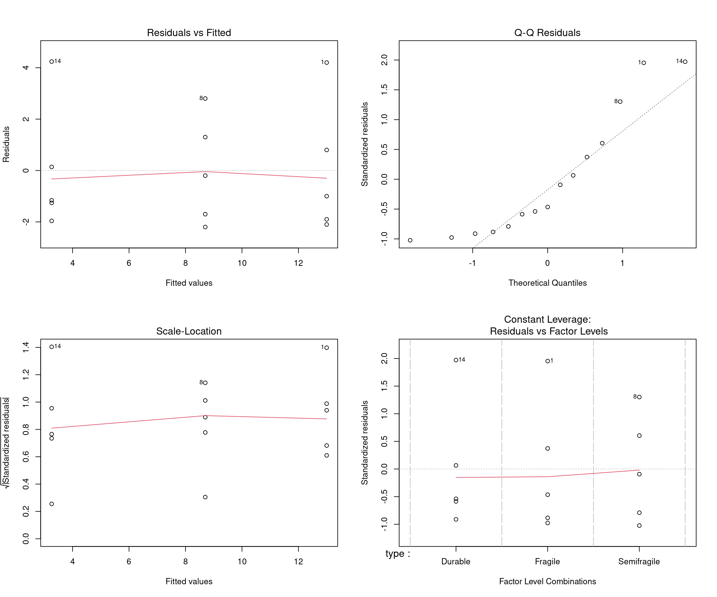

anova(model)

## Analysis of Variance Table
## 
## Response: cost
##           Df  Sum Sq Mean Sq F value    Pr(>F)    
## type       2 238.252 119.126  20.607 0.0001315 ***
## Residuals 12  69.372   5.781                      
## ---
## Signif. codes:  0 '***' 0.001 '**' 0.01 '*' 0.05 '.' 0.1 ' ' 1

summary(model)

## 
## Call:
## lm(formula = cost ~ type)
## 
## Residuals:
##    Min     1Q Median     3Q    Max 
##  -2.20  -1.80  -1.00   1.05   4.24 
## 
## Coefficients:
##                 Estimate Std. Error t value Pr(>|t|)    
## (Intercept)        3.260      1.075   3.032   0.0104 *  
## typeFragile        9.740      1.521   6.405 3.38e-05 ***
## typeSemifragile    5.440      1.521   3.577   0.0038 ** 
## ---
## Signif. codes:  0 '***' 0.001 '**' 0.01 '*' 0.05 '.' 0.1 ' ' 1
## 
## Residual standard error: 2.404 on 12 degrees of freedom
## Multiple R-squared:  0.7745, Adjusted R-squared:  0.7369 
## F-statistic: 20.61 on 2 and 12 DF,  p-value: 0.0001315