4 Introduction to multiple regression
So far, our discussion of the relationship between variables has been restricted to the case of one independent variable (x) that has an influence on the dependent variable (y). However, this simple linear regression model is inadequate for dealing with most problems. Many times, the dependent variable (y) in a problem is influenced by several independent variables. For example, the sales of a product can be influenced by many factors or independent variables: the cost spend on advertising, the time of year, the state of the general economy, the price of the product, the size of the store that sells the product, and the number of competitive products on the market.
For this example there is only one dependent variable (y), as there is for simple linear regression analysis, but there are multiple independent variables \((x_{1}, x_{2}, \cdots,x_{n})\) that influence the dependent variable. Regression analysis with two or more variables is called multiple regression analysis. So why do we need to perform a multiple regression analysis? The answer is simple. We want to get the best predicted values for y by taking all the factors into account that may have an influence on this variable.
This means that more complex models are needed in practical situations, that is, we want to include all the independent variables in the model to make the most accurate predictions for y in the end. So, we will consider problems involving several independent variables using multiple regression analysis. Several multiple regression models will be discussed. Again, we make use of the least squares method to estimate the parameters \((\beta 's)\) of these models. Furthermore, we illustrate how to analyse and interpret computer printouts when multiple regression is applied.
4.1 General form of a multiple regression model
When there are several x variables present, the simple linear regression model can be extended by assuming a linear relationship between each x variable and the dependent y variable. For example, say there are k number of x variables that have an influence on the y variable, then the general form of the multiple regression model for the population is expressed as
\[y = \beta_{0} + \beta_{1}x_{1} + \beta_{2}x_{2} + \cdots + \beta_{n}x_{n} + \epsilon\]
where
y = dependent variable
\(x_{1}, x_{2}, \cdots,x_{n}\) = independent variables
\(\epsilon\) = random error with \(\sim N(0, \sigma^{2})\)
\(\beta_{0}\) = intercept
\(\beta_{1}\) = slope for the variable \(x_{1}\)
\(\beta_{2}\) = slope for the variable \(x_{2}\)
\(\beta_{n}\) = slope for the variable \(x_{n}\)
4.2 First-Order Model
The term first-order is derived from the fact that each x in the model is raised to the first power. Other types of multiple regression models may contain x ’s that are raised to the second power or to the third power (such as \(x_{1}^{2} or x_{2}^{3}\)). The first-order model is also known as the straight-line model, meaning that the relationship between the variable \(x_{1}\) and y is linear (in the form of a straight line), the relationship between the variable \(x_{2}\) and y is linear, and the same for the other x variables.
\[y = \beta_{0} + \beta_{1}x_{1} + \beta_{2}x_{2} + \cdots + \beta_{n}x_{n} + \epsilon\]
This data set was chosen to encourage a discussion about inferences.
Example 4.1 This example is a sample from the Price car prediction dataset. Only continuous variables will be used in this example.
##   Invoice EngineSize Cylinders Horsepower MPG_City MPG_Highway Weight Wheelbase
## 1  33.337        3.5         6        265       17          23   4451       106
## 2  21.761        2.0         4        200       24          31   2778       101
## 3  24.647        2.4         4        200       22          29   3230       105
## 4  30.299        3.2         6        270       20          28   3575       108
## 5  39.014        3.5         6        225       18          24   3880       115
## 6  41.100        3.5         6        225       18          24   3893       115
##   Length
## 1    189
## 2    172
## 3    183
## 4    186
## 5    197
## 6    197
First step
Graphical analysis.
library(lattice)
library(tidyverse)

dato <- gather(dat, "Variables", "X", -Invoice)

xyplot(Invoice ~ X|Variables, data=dato)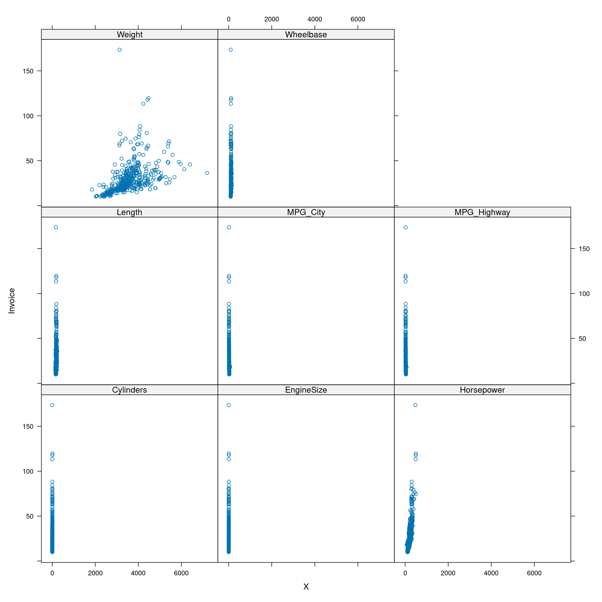
Building the model
model <- lm(Invoice ~ ., data=dat[-335,])Model’s assumptions
par(mfrow=c(2,2))
plot(model)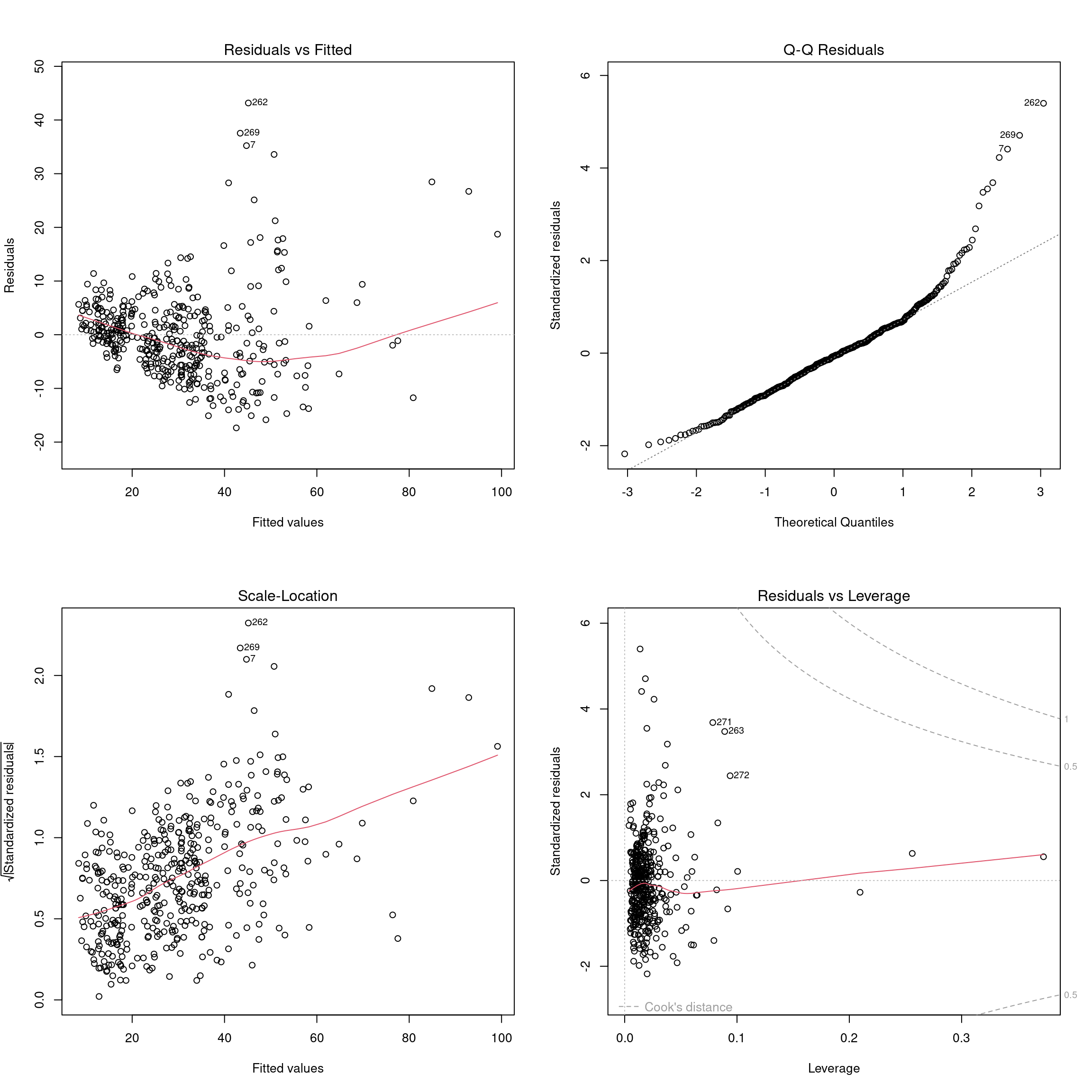
Inference
anova(model)## Analysis of Variance Table
##
## Response: Invoice
## Df Sum Sq Mean Sq F value Pr(>F)
## EngineSize 1 41548 41548 640.9193 < 2.2e-16 ***
## Cylinders 1 13806 13806 212.9766 < 2.2e-16 ***
## Horsepower 1 26260 26260 405.0773 < 2.2e-16 ***
## MPG_City 1 427 427 6.5846 0.01064 *
## MPG_Highway 1 101 101 1.5625 0.21200
## Weight 1 204 204 3.1497 0.07667 .
## Wheelbase 1 2781 2781 42.8969 1.706e-10 ***
## Length 1 97 97 1.4989 0.22153
## Residuals 416 26968 65
## ---
## Signif. codes: 0 '***' 0.001 '**' 0.01 '*' 0.05 '.' 0.1 ' ' 1summary(model)##
## Call:
## lm(formula = Invoice ~ ., data = dat[-335, ])
##
## Residuals:
## Min 1Q Median 3Q Max
## -17.356 -5.082 -0.529 3.534 43.166
##
## Coefficients:
## Estimate Std. Error t value Pr(>|t|)
## (Intercept) 1.815332 8.169867 0.222 0.824268
## EngineSize -4.457566 1.033489 -4.313 2.01e-05 ***
## Cylinders 3.561928 0.647923 5.497 6.73e-08 ***
## Horsepower 0.189988 0.010745 17.682 < 2e-16 ***
## MPG_City -0.311774 0.246245 -1.266 0.206182
## MPG_Highway 0.801318 0.241295 3.321 0.000976 ***
## Weight 0.006462 0.001251 5.164 3.76e-07 ***
## Wheelbase -0.395870 0.119501 -3.313 0.001005 **
## Length -0.080359 0.065636 -1.224 0.221529
## ---
## Signif. codes: 0 '***' 0.001 '**' 0.01 '*' 0.05 '.' 0.1 ' ' 1
##
## Residual standard error: 8.051 on 416 degrees of freedom
## (2 observations deleted due to missingness)
## Multiple R-squared: 0.7596, Adjusted R-squared: 0.755
## F-statistic: 164.3 on 8 and 416 DF, p-value: < 2.2e-164.3 A confidence interval for a single beta parameter in a multiple regression model
The general formula for this confidence interval is given as
\[\hat{\beta_{i}} \pm t_{(n-(k-1); \frac{\alpha}{2}) \times S_{\hat{\beta_{i}}}} \]
where n is the number of observations and k is the total number of parameters of the model.
So if, for example, we want to construct a confidence interval for \(\beta_{2}\) then \(\hat{\beta_{2}}\) is replaced by \(\hat{\beta_{2}}\) and \(S_{\hat{\beta_{i}}}\) is replaced by \(S_{\hat{\beta_{2}}}\) .
Example 4.2 Construct a 90% confidence interval for the horsepower in the Price car dataset
Solution
\[\hat{\beta}_{Horsepower} \pm t_{(428-(9-1); \frac{0.1}{2}) \times S_{\hat{\beta_{Horsepower}}}}\]
\[0.189 \pm 1.648 \times 0.010\]
\[0.189 \pm 1.648 \times 0.010\]
\[0.189 \pm 0.016\]
\[[0.172 ; 0.207]\]
Using R
summary(model)##
## Call:
## lm(formula = Invoice ~ ., data = dat[-335, ])
##
## Residuals:
## Min 1Q Median 3Q Max
## -17.356 -5.082 -0.529 3.534 43.166
##
## Coefficients:
## Estimate Std. Error t value Pr(>|t|)
## (Intercept) 1.815332 8.169867 0.222 0.824268
## EngineSize -4.457566 1.033489 -4.313 2.01e-05 ***
## Cylinders 3.561928 0.647923 5.497 6.73e-08 ***
## Horsepower 0.189988 0.010745 17.682 < 2e-16 ***
## MPG_City -0.311774 0.246245 -1.266 0.206182
## MPG_Highway 0.801318 0.241295 3.321 0.000976 ***
## Weight 0.006462 0.001251 5.164 3.76e-07 ***
## Wheelbase -0.395870 0.119501 -3.313 0.001005 **
## Length -0.080359 0.065636 -1.224 0.221529
## ---
## Signif. codes: 0 '***' 0.001 '**' 0.01 '*' 0.05 '.' 0.1 ' ' 1
##
## Residual standard error: 8.051 on 416 degrees of freedom
## (2 observations deleted due to missingness)
## Multiple R-squared: 0.7596, Adjusted R-squared: 0.755
## F-statistic: 164.3 on 8 and 416 DF, p-value: < 2.2e-16confint(model, level=0.90)## 5 % 95 %
## (Intercept) -11.652895523 15.283559876
## EngineSize -6.161298168 -2.753833672
## Cylinders 2.493810621 4.630044648
## Horsepower 0.172275339 0.207701039
## MPG_City -0.717715061 0.094167769
## MPG_Highway 0.403537281 1.199098806
## Weight 0.004398675 0.008524389
## Wheelbase -0.592869848 -0.198870103
## Length -0.188562588 0.027844045