7 Second-order model for two or more independent variables
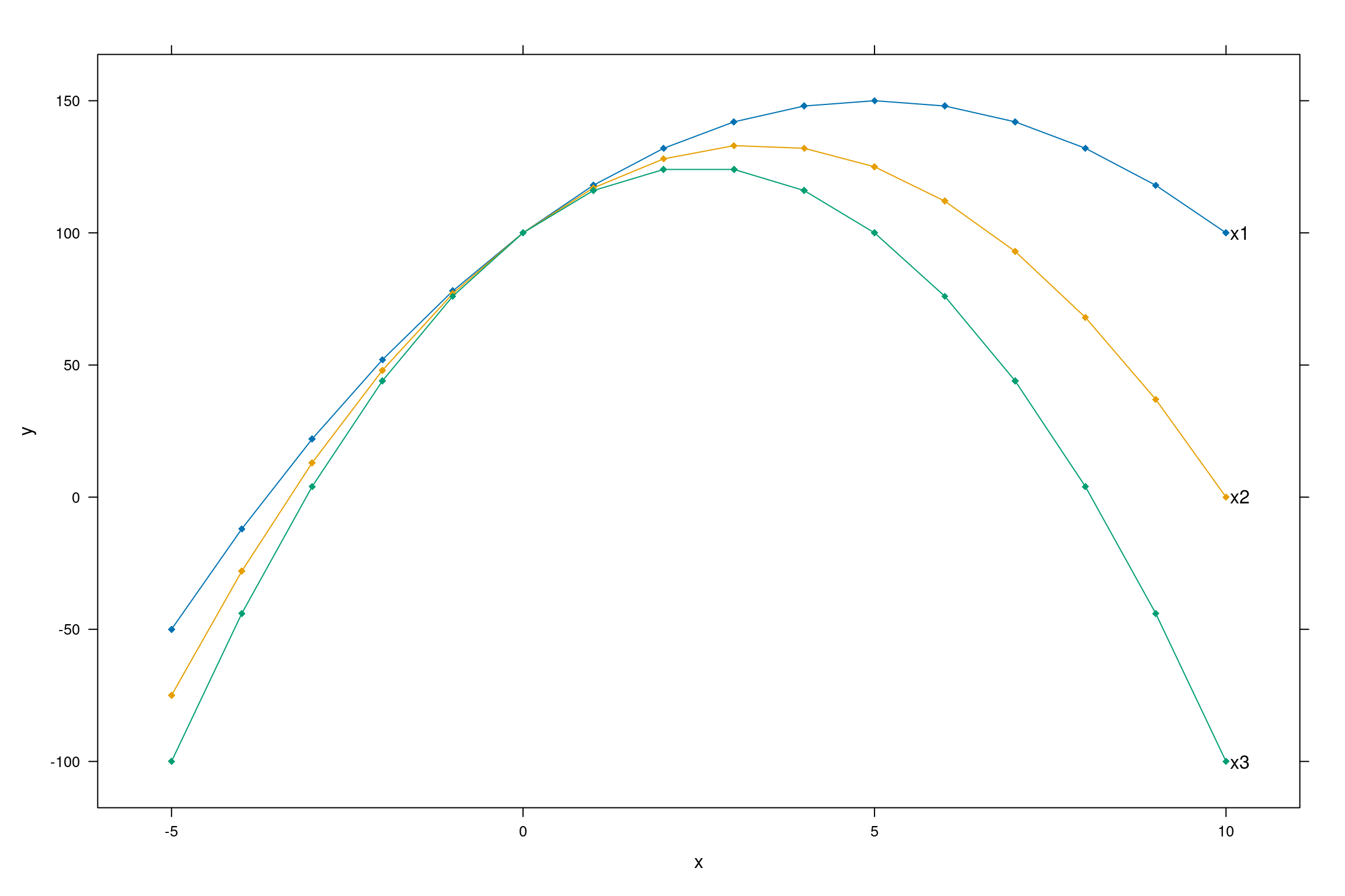
Below is an example of a graph that indicates curvature in the data when more than one x variable have an influence on y.
When we have two quantitative independent variables, namely \(x_{1}\) and \(x_{2}\), that have an influence on y, the second order model is given as
\[E(y) = \beta_{0} + \beta_{1}x_{1} + \beta_{2} x_{2} + \beta_{3} x_{1} x_{2} + \beta_{4} x_{1}^{2} + \beta_{5} x_{1}^{2}\]
Now let me explain step by step how this model is constructed.
Step 1: Write down the original model that includes the two x variables. That is
\[E(y) = \beta_{0} + \beta_{1}x_{1} + \beta_{2} x_{2}\]
Step 2: Add the interaction term between \(x_{1}\) and \(x_{2}\) to the model in Step 1
\[E(y) = \beta_{0} + \beta_{1}x_{1} + \beta_{2} x_{2} + \beta_{3} x_{1} x_{2}\]
Step 3: Add the quadratic terms of \(x_{1}\) and \(x_{2}\) to the model in Step 2
\[E(y) = \beta_{0} + \beta_{1}x_{1} + \beta_{2} x_{2} + \beta_{3} x_{1} x_{2} + \beta_{4} x_{1}^{2} + \beta_{5} x_{1}^{2}\]
Example 7.1 An express delivery service bases the cost (y) for shipping a package on the package weight (x1) and distance shipped (x2). So here we have two factors, package weight (x1) and distance shipped (x2) that have an influence on the cost of shipping (or courier) the package (y). The cost will most likely increase if the weight increases and also if the distance shipped increases. The cost is given in R100, the weight in kilogram and the distance in kilometers.
The data consist of 20 pairs of observations, thus n = 20. A graph of the data indicates curvature in the data.
Write down an appropriate model for the data.
Fit the model to the data and give the prediction equation.
Find the value of the coefficient of determination and interpret the value.
Predict the shipping cost when the weight of the package is 5 kilograms and the distance shipped is 100 kilometers.
Solution
weight <- c(5.9, 3.2, 4.4, 6.6, 0.75, 0.70, 6.5, 4.5, 0.6,
            7.5, 5.1, 2.4, 0.3, 6.2, 2.7, 3.5, 4.1, 8.1, 7.0, 1.1)

distance <- c(47, 145, 202, 160, 280, 80, 240, 53, 100, 190,
             240, 209, 160, 115, 45, 250, 95, 160, 260, 90)

cost <- c(2.6, 3.9, 8.0, 9.2, 4.4, 1.5, 14.5, 1.9, 1, 14.0,
11, 5, 2, 6, 1.1, 8, 3.3, 12.1, 15.5, 1.7)library(lattice)
library(gridExtra)
p1 <- xyplot(cost ~ weight, xlab="Weight (Kg)", ylab="Cost (R100)", pch=19)
p2 <- xyplot(cost ~ distance, xlab="Distance (Km)", pch=19, ylab="", col="red")
grid.arrange(p1,p2, ncol=2)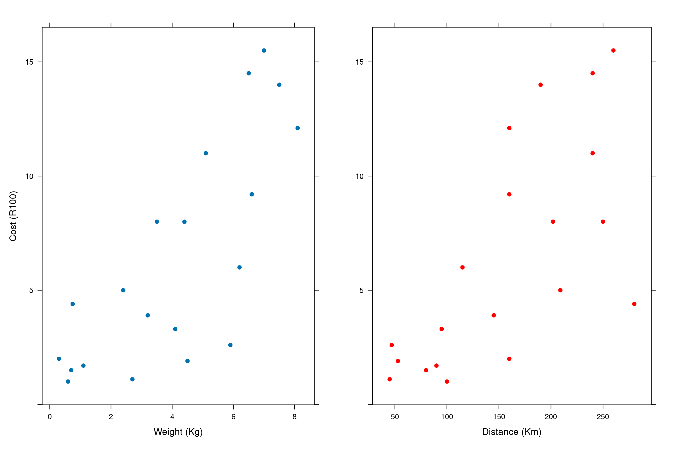
mod <- lm(cost ~ weight + distance + weight*distance + I(weight^2) + I(distance^2))

summary(mod)
##
## Call:
## lm(formula = cost ~ weight + distance + weight * distance + I(weight^2) +
## I(distance^2))
##
## Residuals:
## Min 1Q Median 3Q Max
## -0.86027 -0.19898 -0.00885 0.16531 0.94396
##
## Coefficients:
## Estimate Std. Error t value Pr(>|t|)
## (Intercept) 8.270e-01 7.023e-01 1.178 0.258588
## weight -6.091e-01 1.799e-01 -3.386 0.004436 **
## distance 4.021e-03 7.998e-03 0.503 0.622999
## I(weight^2) 8.975e-02 2.021e-02 4.442 0.000558 ***
## I(distance^2) 1.507e-05 2.243e-05 0.672 0.512657
## weight:distance 7.327e-03 6.374e-04 11.495 1.62e-08 ***
## ---
## Signif. codes: 0 '***' 0.001 '**' 0.01 '*' 0.05 '.' 0.1 ' ' 1
##
## Residual standard error: 0.4428 on 14 degrees of freedom
## Multiple R-squared: 0.9939, Adjusted R-squared: 0.9918
## F-statistic: 458.4 on 5 and 14 DF, p-value: 5.371e-15anova(mod)## Analysis of Variance Table
##
## Response: cost
## Df Sum Sq Mean Sq F value Pr(>F)
## weight 1 270.553 270.553 1380.0008 2.168e-15 ***
## distance 1 143.631 143.631 732.6164 1.722e-13 ***
## I(weight^2) 1 8.979 8.979 45.7989 9.060e-06 ***
## I(distance^2) 1 0.273 0.273 1.3939 0.2574
## weight:distance 1 25.904 25.904 132.1280 1.622e-08 ***
## Residuals 14 2.745 0.196
## ---
## Signif. codes: 0 '***' 0.001 '**' 0.01 '*' 0.05 '.' 0.1 ' ' 1par(mfrow=c(2,2))
plot(mod)
0.827 - 0.609*(5) + 0.004*(100) + 0.007*(5)*(100) + 0.089*(5)^2 + 0.000015*(100)^2## [1] 4.057When curvature is expected, we have to write down a second-order model for the two x variables. The model is \(E(y) = \beta_{0} + \beta_{1} x_{1} + \beta_{2} x_{2} + \beta_{3} x_{1} x_{2} + \beta_{4} x_{1}^{2} + \beta_{5} x_{2}^{2}\)
\(\hat{y} = 0.827 - 0.609 x_{1} + 0.004 x_{2} + 0.007 x_{1} x_{2} + 0.089 x_{1}^{2} + 0.000015 x_{2}^{2}\)
\(R^{2}=0.9918\). The second-order model explain 99.18% of the changes in the shipping cost (y).
To predict the cost (y), just use the estimated equation.
\(\hat{y} = 0.827 - 0.609 (5) + 0.004 (100) + 0.007 (5)(100) + 0.089 (5)^{2} + 0.000015 (100)^{2} = 4.057\)