9 A Test for Comparing Nested Models
So why do we have to perform this test? Well, as you know by now, there are many different multiple regression models that can be fitted to a data set (e.g. the straight-line model, the interaction model, the quadratic model and models with qualitative variables). But, unfortunately, it is not always that easy to decide on which model to fit to a data set (the scattergrams, which usually give a good indication of which model to use, can sometimes be misleading or not easy to read).
So, in reality, it sometimes happens that we have to choose between two possible models that can be fitted to a data set. Now what we want to know is which one of the two models is the best model to fit to the data or which one of the two models will give the best predicted value of y. In this lecture I shall discuss a hypothesis test (a F test) that will do just that. It is important to remember that we can only use this test when the models are nested. Let me explain what “nested” means by means of an example.
Example 9.1 Suppose you have collected data on a y variable, and two independent variables (x1 and x2) that have an influence on the y variable. According to the characteristics of the data set as well as the scattergram of the data, we are not sure whether to fit the interaction model or the curvilinear (second-order) model to the data. Will the second-order model provide better predictions of y than the interaction model? To answer this question, we first have to examine the two models. By now, you should be able to write down the two types of models for the two x variables, so lets have a look at them:
Interaction model: \(E(y) = \beta_{0} + \beta_{1} x_{1} + \beta_{2} x_{2} + \beta_{3} x_{1} x_{2}\)
Second-order model: \(E(y) = \beta_{0} + \beta_{1} x_{1} + \beta_{2} x_{2} + \beta_{3} x_{1} x_{2} + \beta_{4} x_{1}^{2} + \beta_{5} x_{2}^{2}\)
This is a typical example of nested models. Why? Because all the terms of the interaction model also appears in the second-order model. The second-order model just has two extra terms So two models are called nested models when ALL the terms of one model appears in the other model, and the other model have some extra terms.
We also have some other terminology to consider. The shorter or simpler model of the two is called the reduced model. In this case the reduced model will be the interaction model. On the other hand, the longer or more complex model of the two is called the complete model. In this case the complete model will be the second-order model.
Before we discuss the general steps to follow for the hypothesis test for nested models, I just want to explain what the null and alternative hypotheses will look like for this specific example. What we actually want to know is whether it is necessary to include the quadratic terms, \(\beta_{4} x_{1}^{2}\) and \(\beta_{5} x_{2}^{2}\) or not (the extra terms that appears in the second-order model but not in the interaction model). It is clear that the second-order model without the quadratic terms is exactly the same as the interaction model. Therefore we are only interested in whether the additional terms that appear in the second-order model, but not in the interaction model, are important to include or not. So when we perform the test, we test only for \(\beta_{4} x_{1}^{2}\) and \(\beta_{5} x_{2}^{2}\). The null and alternative hypotheses will then be as follows:
\(H_{0}: \beta_{4}=\beta_{5}=0\)
\(H_{a}:\) At least one of the betas differ from zero
Example 9.2 We want to know whether the additional terms in the complete model (i.e. those terms that does not appear in the reduced model), is important to include or not.
\(E(y) = \beta_{0} + \beta_{1}x\) (reduced model)
\(E(y) = \beta_{0} + \beta_{1}x + \beta_{2} x^{2} + \beta_{3} x^{3}\) (complete model)
Then, the hypotheses are:
\(H_{0}: \beta_{2}=\beta_{3}=0\)
\(H_{a}:\) At least one of the betas differ from zero
9.1 The general F test for comparing nested models
Again, as usual, we are going to follow six steps to perform this test. However, it is important to, first of all, write down the two models that we compare in order to be able to perform the six steps of the hypothesis test. We must also remember that both models will be fitted to the same data and therefore there will be two printouts (one for each model) that we will use to perform the test. So in general our two models will be:
Now we can begin with the six steps
Step 1:
\(H_{0}: \beta_{0}=\beta_{2}=\cdots=\beta_{n}=0\)
\(H_{a}:\) At least one of the betas differ from zero
Step 2:
Specify \(\alpha\)
Step 3:
Calculate the test statistic.
\[F = \frac{SSE_{R}-SSE_{C}}{df_{R}-df_{C}} / MSE_{C}\]
where
\(df_{R}\) = degrees of freedom for the reduced model
\(df_{C}\) = degrees of freedom for the complete model
\(SSE_{R}\) = the SSE value for the reduced model
\(SSE_{C}\) = the SSE value for the complete model
\(MSE_{C}\) = the MSE value for the complete model
Step 4:
Find the F table value which is \(F_{(k-g; n-(k+1);\alpha)}\)
Step 5:
Conclusion
Example 9.3 A dataset containing the prices and other attributes of almost 54,000 diamonds. The variables length (x), width (y) and depth (z) will be used for this example.
data(diamonds)

head(diamonds)
## # A tibble: 6 × 10
## carat cut color clarity depth table price x y z
## <dbl> <ord> <ord> <ord> <dbl> <dbl> <int> <dbl> <dbl> <dbl>
## 1 0.23 Ideal E SI2 61.5 55 326 3.95 3.98 2.43
## 2 0.21 Premium E SI1 59.8 61 326 3.89 3.84 2.31
## 3 0.23 Good E VS1 56.9 65 327 4.05 4.07 2.31
## 4 0.29 Premium I VS2 62.4 58 334 4.2 4.23 2.63
## 5 0.31 Good J SI2 63.3 58 335 4.34 4.35 2.75
## 6 0.24 Very Good J VVS2 62.8 57 336 3.94 3.96 2.48library(lattice)
library(gridExtra)
library(tidyr)
dat.graf <- pivot_longer(diamonds, cols=c("x","y","z"), names_to="Variable", values_to="Resp")
xyplot(price ~ Resp|Variable, data=dat.graf, ylab="Price (US dollars)", xlab="mm",
strip=strip.custom(factor.levels=c("Length","Width","Depth")),
scales=list(relation="free"), alternating=1)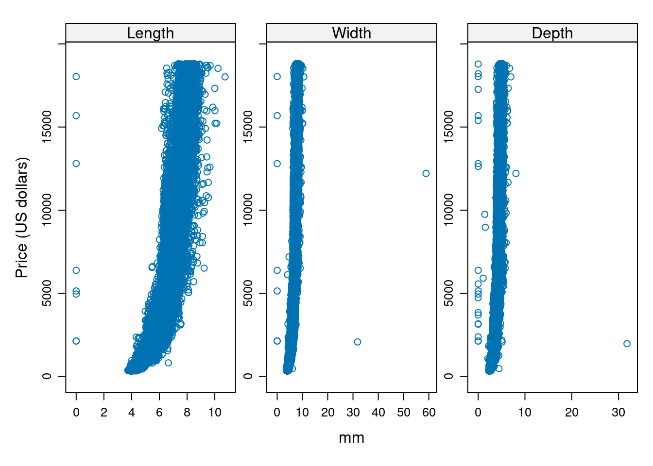
Models
\(E(y) = \beta_{0} + \beta_{1} x + \beta_{2} y + \beta_{3} z\) Reduced model
\(E(y) = \beta_{0} + \beta_{1} x + \beta_{2} y + \beta_{3} z + \beta_{4} x^{2} + \beta_{5} y^{2} + \beta_{6} z^{2}\) Complete model
\(\alpha\) = 0.05
Hypotheses
\(H_{0}: \beta_{4}=\beta_{5}=\beta_{6}=0\)
\(H_{a}:\) At least one parameter differ from zero
reduced.model <- lm(price ~ x + y + z, data=diamonds)

complete.model <- lm(price ~ x + y + z + I(x^2) + I(y^2) + I(z^2), data=diamonds)anova(reduced.model)## Analysis of Variance Table
##
## Response: price
## Df Sum Sq Mean Sq F value Pr(>F)
## x 1 6.7152e+11 6.7152e+11 194015.499 < 2.2e-16 ***
## y 1 1.9408e+08 1.9408e+08 56.073 7.090e-14 ***
## z 1 7.8047e+07 7.8047e+07 22.549 2.053e-06 ***
## Residuals 53936 1.8668e+11 3.4612e+06
## ---
## Signif. codes: 0 '***' 0.001 '**' 0.01 '*' 0.05 '.' 0.1 ' ' 1summary(reduced.model)##
## Call:
## lm(formula = price ~ x + y + z, data = diamonds)
##
## Residuals:
## Min 1Q Median 3Q Max
## -10958 -1269 -187 975 32147
##
## Coefficients:
## Estimate Std. Error t value Pr(>|t|)
## (Intercept) -14113.05 41.76 -337.936 < 2e-16 ***
## x 2790.32 40.98 68.082 < 2e-16 ***
## y 218.79 31.56 6.932 4.21e-12 ***
## z 225.91 47.57 4.749 2.05e-06 ***
## ---
## Signif. codes: 0 '***' 0.001 '**' 0.01 '*' 0.05 '.' 0.1 ' ' 1
##
## Residual standard error: 1860 on 53936 degrees of freedom
## Multiple R-squared: 0.7825, Adjusted R-squared: 0.7825
## F-statistic: 6.47e+04 on 3 and 53936 DF, p-value: < 2.2e-16anova(complete.model)## Analysis of Variance Table
##
## Response: price
## Df Sum Sq Mean Sq F value Pr(>F)
## x 1 6.7152e+11 6.7152e+11 304203.217 < 2.2e-16 ***
## y 1 1.9408e+08 1.9408e+08 87.918 < 2.2e-16 ***
## z 1 7.8047e+07 7.8047e+07 35.356 2.763e-09 ***
## I(x^2) 1 6.6273e+10 6.6273e+10 30021.954 < 2.2e-16 ***
## I(y^2) 1 1.0595e+09 1.0595e+09 479.951 < 2.2e-16 ***
## I(z^2) 1 2.9383e+08 2.9383e+08 133.105 < 2.2e-16 ***
## Residuals 53933 1.1906e+11 2.2075e+06
## ---
## Signif. codes: 0 '***' 0.001 '**' 0.01 '*' 0.05 '.' 0.1 ' ' 1summary(complete.model)##
## Call:
## lm(formula = price ~ x + y + z + I(x^2) + I(y^2) + I(z^2), data = diamonds)
##
## Residuals:
## Min 1Q Median 3Q Max
## -21990.4 -548.3 -34.1 290.4 12832.9
##
## Coefficients:
## Estimate Std. Error t value Pr(>|t|)
## (Intercept) 12762.271 159.201 80.17 <2e-16 ***
## x -8904.714 109.290 -81.48 <2e-16 ***
## y 1945.605 88.890 21.89 <2e-16 ***
## z 1132.444 70.003 16.18 <2e-16 ***
## I(x^2) 836.292 4.916 170.12 <2e-16 ***
## I(y^2) -31.520 1.481 -21.28 <2e-16 ***
## I(z^2) -30.979 2.685 -11.54 <2e-16 ***
## ---
## Signif. codes: 0 '***' 0.001 '**' 0.01 '*' 0.05 '.' 0.1 ' ' 1
##
## Residual standard error: 1486 on 53933 degrees of freedom
## Multiple R-squared: 0.8613, Adjusted R-squared: 0.8613
## F-statistic: 5.583e+04 on 6 and 53933 DF, p-value: < 2.2e-16anova(reduced.model, complete.model)## Analysis of Variance Table
##
## Model 1: price ~ x + y + z
## Model 2: price ~ x + y + z + I(x^2) + I(y^2) + I(z^2)
## Res.Df RSS Df Sum of Sq F Pr(>F)
## 1 53936 1.8668e+11
## 2 53933 1.1906e+11 3 6.7626e+10 10212 < 2.2e-16 ***
## ---
## Signif. codes: 0 '***' 0.001 '**' 0.01 '*' 0.05 '.' 0.1 ' ' 1Conclusion
We can reject the \(H_{0}\) hypotheses. Therefore, the full model must be selected with a 5% error by F test.