11 Extra exercises
11.1 Multivariate regression model with quantitatives independent variables
Example 11.1 Limestone
limestone <- rep(c(0,0.25,2,3.72), each=25)

organic <- rep(c(0,5,10,20,40), each=5)

msf <- c(0.45,0.46,0.51,0.90,0.79,5.58,5.38,5.21,5.16,6.39,5.74,5.38,6.01,4.99,5.99,6.65,6.27,6.19,6.82,
         7.03,6.61,7.97,7.33,8.21,6.66,0.95,1.27,5.62,6.08,1.01,5.13,8.56,4.11,5.64,4.97,5.62,6.78,5.35,
                 5.22,6.15,6.26,6.81,5.57,6.32,6.31,7.91,7.05,6.32,7.88,7.03,2.01,5.49,2.44,1.18,3.93,6.07,5.22,
                 6.28,5.94,5.37,5.76,6.68,6.25,5.83,6.31,6.55,6.22,6.93,6.85,6.68,6.49,6.83,7.05,7.05,6.32,1.31,
                 1.02,1.33,1.22,1.86,4.64,4.95,6.24,5.61,6.30,6.41,5.43,5.57,6.28,6.43,6.29,6.70,6.12,6.27,6.68,
                 3.48,2.21,3.95,6.56,6.77)

dat <- data.frame(limestone=limestone, organic=organic, msf=msf)
Visual analysis
library(lattice)
library(latticeExtra)
library(tidyr)


xyplot(msf ~ organic|factor(limestone), data=dat, ylab="Dry leaf matter (g)", type=c("a","p"),
       scales=list(alternating=1), xlab=expression(paste('Organic matter (g/dm'^{3},')')))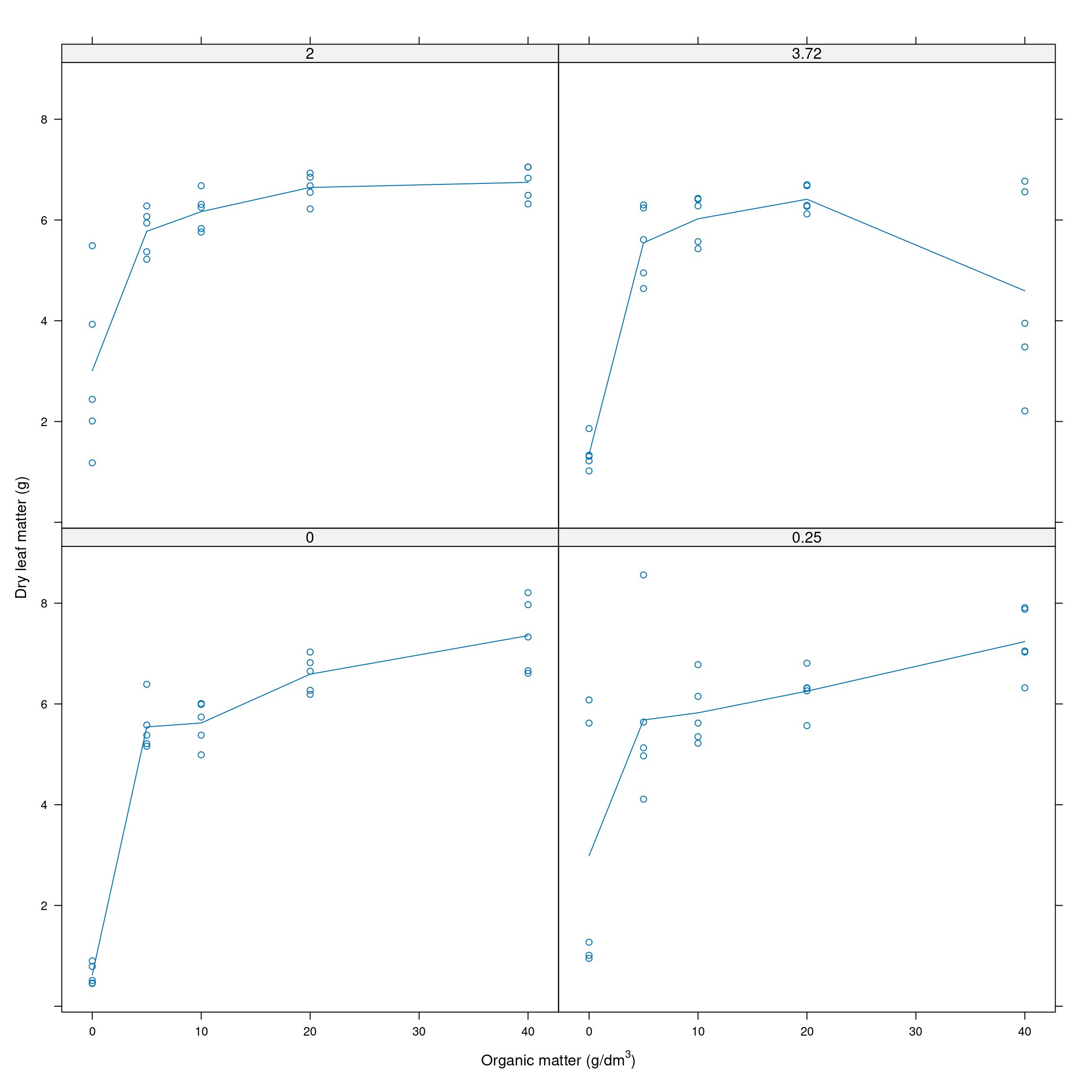
Figure 11.1: Dry leaf matter by organic matter at different levels of limestone
xyplot(msf ~ limestone|factor(organic), data=dat, ylab="Dry leaf matter (g)", type=c("a","p"),
       scales=list(alternating=1), xlab=expression(paste('Limestone (g/dm'^{3},')')))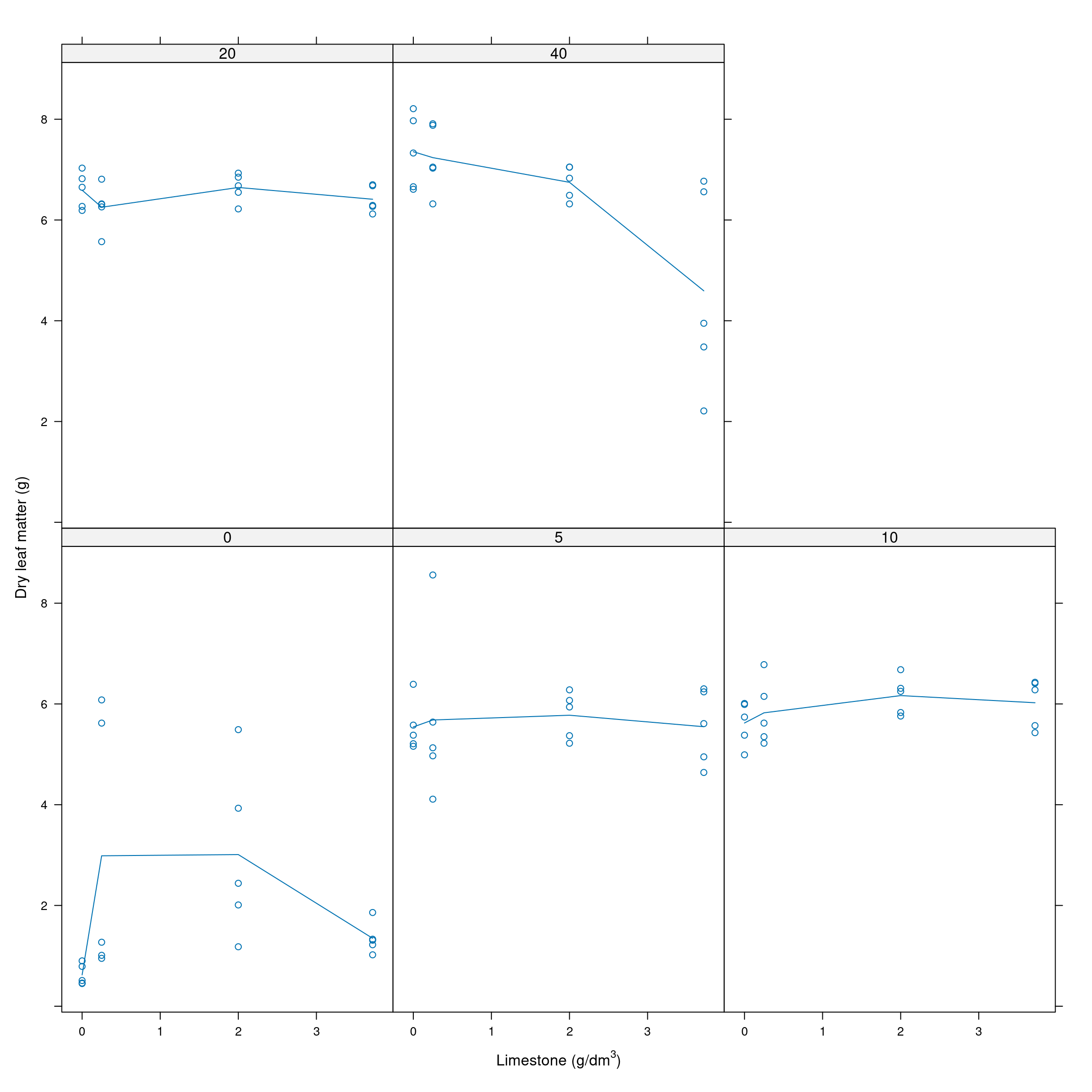
Figure 11.2: Dry leaf matter by limestone at different levels of organic matter
library(scatterplot3d)

funct <- colorRamp(c("blue","red"))

mscol <- with(dat, (msf - min(msf)) / diff(range(msf)))

cols <- funct(mscol)


col.f <-  rgb(cols, maxColorValue=256)


cloud(msf ~ organic + limestone, data=dat,
           col=col.f,
           scales = list(arrows = FALSE, y=list(at=c(0.25,2,3.72))),
           screen = list(z = 30, x = -60),
           xlab=list(expression(paste('Organic matter (g/dm'^{3},')')), rot=20),
           ylab=list(expression(paste('Limestone (g/dm'^{3},')')), rot=-48),
           zlab=list('Dry matter (g)', rot=95),
           par.box = list(col=c(1,1,NA,NA,1,NA,1,1,1)))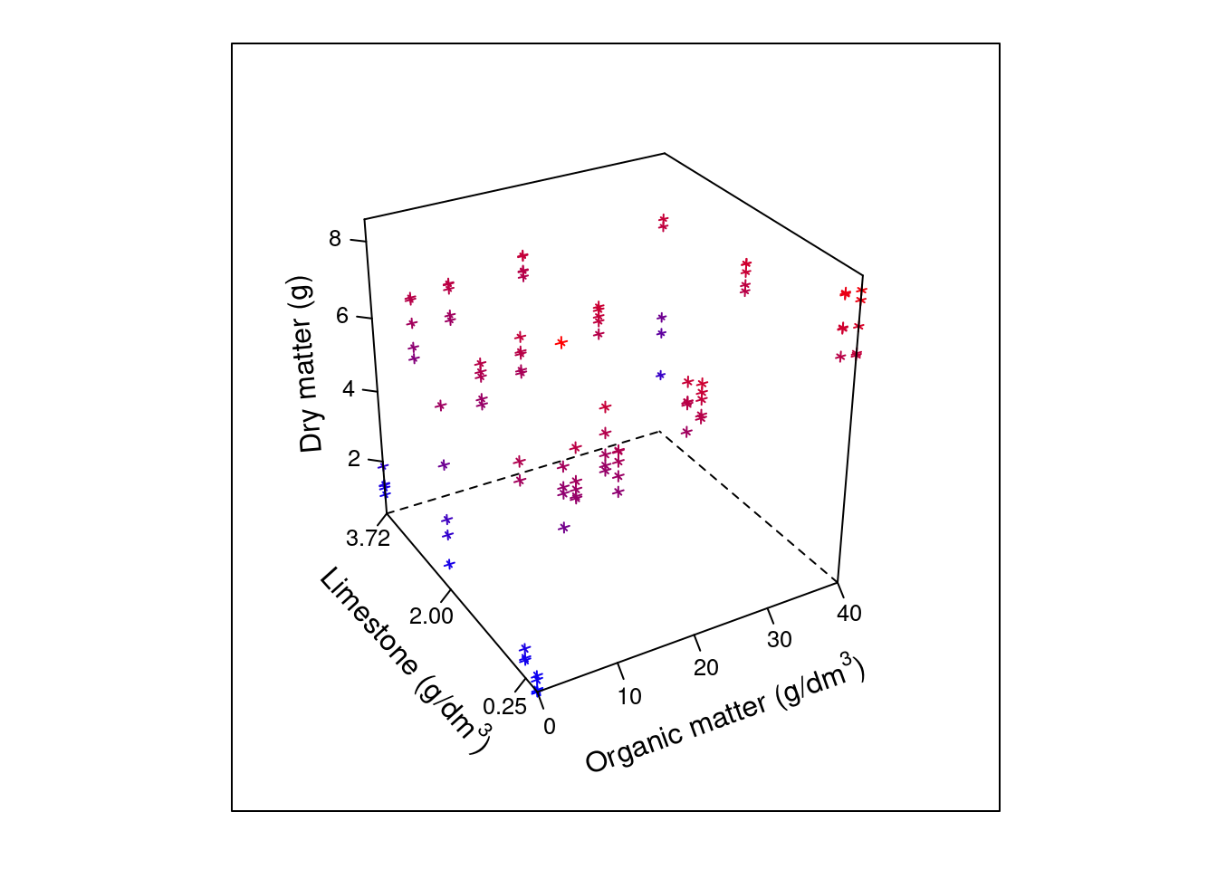
Full Model
model.full <- lm(msf ~ limestone*organic + I(organic^2) + I(limestone^2), data=dat)
anova(model.full)
## Analysis of Variance Table
##
## Response: msf
## Df Sum Sq Mean Sq F value Pr(>F)
## limestone 1 3.365 3.365 1.9812 0.162564
## organic 1 123.834 123.834 72.9086 2.338e-13 ***
## I(organic^2) 1 104.419 104.419 61.4776 6.881e-12 ***
## I(limestone^2) 1 8.215 8.215 4.8366 0.030314 *
## limestone:organic 1 14.265 14.265 8.3986 0.004673 **
## Residuals 94 159.658 1.698
## ---
## Signif. codes: 0 '***' 0.001 '**' 0.01 '*' 0.05 '.' 0.1 ' ' 1summary(model.full)##
## Call:
## lm(formula = msf ~ limestone * organic + I(organic^2) + I(limestone^2),
## data = dat)
##
## Residuals:
## Min 1Q Median 3Q Max
## -2.6133 -0.9845 -0.0151 0.8648 4.2209
##
## Coefficients:
## Estimate Std. Error t value Pr(>|t|)
## (Intercept) 2.4585670 0.3243515 7.580 2.41e-11 ***
## limestone 0.8884810 0.3610980 2.460 0.01570 *
## organic 0.3708702 0.0362838 10.221 < 2e-16 ***
## I(organic^2) -0.0064387 0.0008212 -7.841 6.88e-12 ***
## I(limestone^2) -0.2039747 0.0927482 -2.199 0.03031 *
## limestone:organic -0.0178137 0.0061468 -2.898 0.00467 **
## ---
## Signif. codes: 0 '***' 0.001 '**' 0.01 '*' 0.05 '.' 0.1 ' ' 1
##
## Residual standard error: 1.303 on 94 degrees of freedom
## Multiple R-squared: 0.6141, Adjusted R-squared: 0.5936
## F-statistic: 29.92 on 5 and 94 DF, p-value: < 2.2e-16Model selection
library(MASS)##
## Attaching package: 'MASS'## The following object is masked from 'package:dplyr':
##
## selectmod.sel <- stepAIC(model.full)## Start: AIC=58.79
## msf ~ limestone * organic + I(organic^2) + I(limestone^2)
##
## Df Sum of Sq RSS AIC
## <none> 159.66 58.786
## - I(limestone^2) 1 8.215 167.87 61.804
## - limestone:organic 1 14.265 173.92 65.344
## - I(organic^2) 1 104.419 264.08 107.107Final model
\[E(y) = 2.458 + 0.888*limestone + 0.371*organic - 0.006^{2}*organic - 0.204^{2}*limestone - 0.017*organic*limestone\]
Predictions
limestone <- c(seq(0,3.76,0.12), 0.94)
organic <- c(seq(0,40,2.5), 29.58)


graf.f <- expand.grid(limestone=limestone,organic=organic)


pred <- predict(model.full, newdata=graf.f)

graf.f[["Pred"]] <- predwireframe(Pred ~ organic + limestone, data=graf.f,
drape=TRUE, colorkey=TRUE, #par.settings = standard.theme(color = FALSE),
col='transparent',
scales = list(arrows = FALSE, y=list(at=c(0.25,2,3.72))),
screen = list(z = 30, x = -60),
xlab=list(expression(paste('Organic matter (g/dm'^{3},')')), rot=20),
ylab=list(expression(paste('Limestone (g/dm'^{3},')')), rot=-48),
zlab=list('Dry leaf matter', rot=95),
par.box = list(col=c(1,1,NA,NA,1,NA,1,1,1)))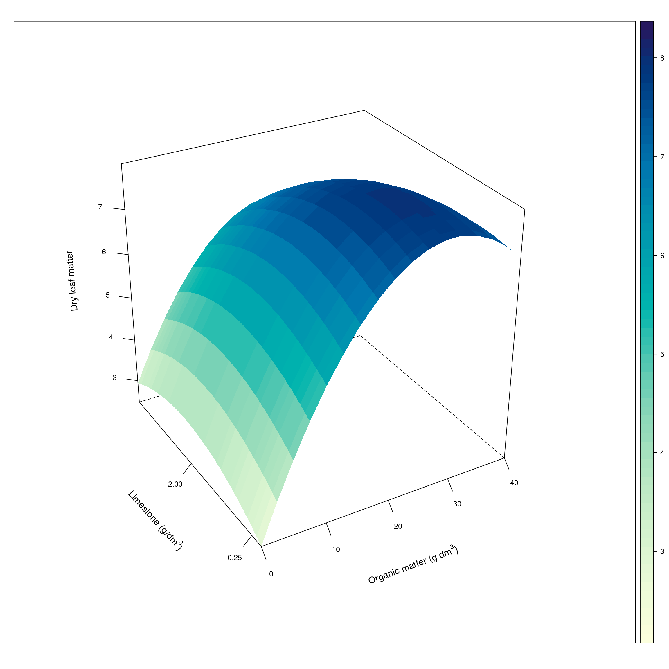
Finding of maximum points of the equation
Use of the online calculator is recommended: Critical Point Calculator
x (limestone) = 0.94
y (organic matter) = 29.58
Therefore, the maximum recommended concentration for limestone and organic matter is 0.94 \((g/dm^{3})\) and 29.58 \((g/dm^{3})\) respectively, whose maximum expected dry leaf matter is 7.95g.
11.2 Regression model with quantitative and qualitative variables
Example 11.2 Analysis of the growth of fungal hyphae.
The experiment was conducted to determine the effects of the duration of water exposure in a 24-hour period in two different fungi.
Questions:
Do the two fungi being tested have the same growth pattern? Can I use the same model for both fungi?
water.time <- rep(c(2,4,6,8,12,16,20,24), each=6)

fungi <- rep(c("S1","S2"), each=length(water.time))

fungi.l <- c(1.50,1.50,1.37,1.89,1.00,1.00,1.57,1.63,1.30,1.48,1.00,1.00,1.53,1.72,1.65,2.18,1.78,1.77,2.64,
            3.02,2.57,2.82,2.10,2.51,4.12,2.44,3.37,4.05,3.93,2.94,3.64,3.27,3.62,2.92,4.26,3.54,2.78,3.13,
                        2.70,2.88,2.48,3.80,3.20,3.30,3.64,3.15,2.65,3.26,1.00,1.20,1.34,1.34,1.24,1.38,1.12,1.17,1.18,
                        1.14,1.18,1.16,1.00,1.35,1.10,1.06,1.35,1.17,2.56,2.70,2.74,2.40,2.44,2.80,1.54,1.03,2.00,1.00,
                        2.05,1.39,4.81,3.08,3.25,3.30,3.36,2.97,2.00,1.97,2.26,2.07,1.90,2.04,1.95,2.50,2.60,2.21,2.30,2.56)

data <- data.frame(water=water.time, fungi=fungi, resp=fungi.l)
head(data)
## water fungi resp
## 1 2 S1 1.50
## 2 2 S1 1.50
## 3 2 S1 1.37
## 4 2 S1 1.89
## 5 2 S1 1.00
## 6 2 S1 1.00library(lattice)
xyplot(resp ~ water, groups=fungi, data=data, type=c("smooth","p"), auto.key=list(space="top", columns=2))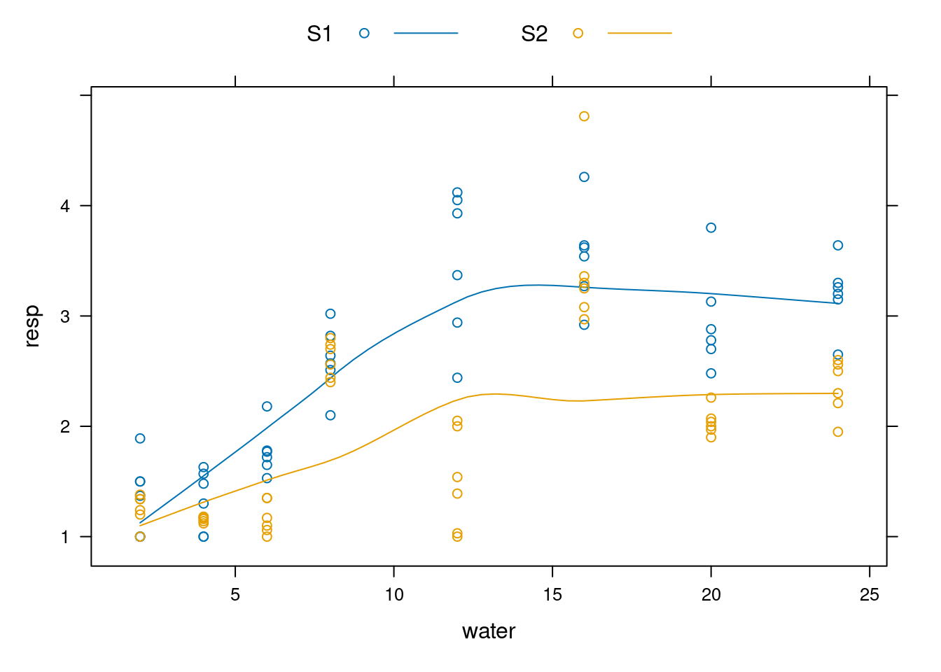
Model selection
library(MASS)


model.f <- lm(resp ~ fungi*water + fungi*I(water^2), data=data)
summary(model.f)
##
## Call:
## lm(formula = resp ~ fungi * water + fungi * I(water^2), data = data)
##
## Residuals:
## Min 1Q Median 3Q Max
## -1.30946 -0.40215 -0.05681 0.34781 2.31039
##
## Coefficients:
## Estimate Std. Error t value Pr(>|t|)
## (Intercept) 0.415141 0.258053 1.609 0.1112
## fungiS2 0.169263 0.364942 0.464 0.6439
## water 0.341045 0.050322 6.777 1.24e-09 ***
## I(water^2) -0.009646 0.001910 -5.050 2.30e-06 ***
## fungiS2:water -0.125127 0.071166 -1.758 0.0821 .
## fungiS2:I(water^2) 0.003632 0.002701 1.345 0.1821
## ---
## Signif. codes: 0 '***' 0.001 '**' 0.01 '*' 0.05 '.' 0.1 ' ' 1
##
## Residual standard error: 0.579 on 90 degrees of freedom
## Multiple R-squared: 0.6378, Adjusted R-squared: 0.6176
## F-statistic: 31.69 on 5 and 90 DF, p-value: < 2.2e-16model.s <- stepAIC(model.f)## Start: AIC=-99.11
## resp ~ fungi * water + fungi * I(water^2)
##
## Df Sum of Sq RSS AIC
## - fungi:I(water^2) 1 0.60615 30.779 -99.200
## <none> 30.173 -99.110
## - fungi:water 1 1.03640 31.210 -97.867
##
## Step: AIC=-99.2
## resp ~ fungi + water + I(water^2) + fungi:water
##
## Df Sum of Sq RSS AIC
## <none> 30.779 -99.200
## - fungi:water 1 1.3351 32.115 -97.124
## - I(water^2) 1 11.2653 42.045 -71.259summary(model.s)##
## Call:
## lm(formula = resp ~ fungi + water + I(water^2) + fungi:water,
## data = data)
##
## Residuals:
## Min 1Q Median 3Q Max
## -1.41087 -0.40119 -0.04103 0.38231 2.22590
##
## Coefficients:
## Estimate Std. Error t value Pr(>|t|)
## (Intercept) 0.611694 0.213600 2.864 0.0052 **
## fungiS2 -0.223843 0.219398 -1.020 0.3103
## water 0.294420 0.036630 8.038 3.20e-12 ***
## I(water^2) -0.007830 0.001357 -5.771 1.08e-07 ***
## fungiS2:water -0.031876 0.016044 -1.987 0.0500 *
## ---
## Signif. codes: 0 '***' 0.001 '**' 0.01 '*' 0.05 '.' 0.1 ' ' 1
##
## Residual standard error: 0.5816 on 91 degrees of freedom
## Multiple R-squared: 0.6305, Adjusted R-squared: 0.6142
## F-statistic: 38.82 on 4 and 91 DF, p-value: < 2.2e-16The stepwise methodology using the AIC criteria for model selection presented the following models:
Fungi S1: \(E(y) = \beta_{0} + \beta_{1}X + \beta_{2c}x^{2}\)
Fungi S2: \(E(y) = \beta_{0} + \beta_{1}X + \beta_{2c}X^{2}\)
Equations
Fungi S1: \(0.611694 + 0.294420X - 0.0078x^{2}\)
\(\beta_{0}\) for S2 is \((Intercept) - fungiS2\) = \(0.611694-0.223843=0.3878\)
\(\beta_{1}\) for S2 is \(water - fungiS2:water\) = \(0.294420-0.031876=0.2625\)
Fungi S2: \(0.3878 + 0.2625X - 0.0078x^{2}\)
Maximum
S1: 18.87 hours
\(f_{s1}(18.87) = 0.611694 + 0.294420(18.87) - 0.0078(18.87)^{2} = 3.39\)
S2: 16.82 hours
\(f_{s2}(16.82) = 0.3878 + 0.2625(16.82) - 0.0078(16.82)^{2} = 2.59\)
Predictions
library(tactile)
library(latticeExtra)


pred <- predict(model.s, interval="confidence")

xyplot(pred[,1] ~ water, groups=fungi, data=data, type="l",
       ylim=c(0,4), xlab="Water (hours)", ylab="Length (mm)",
       lower=pred[,2], upper=pred[,3],
             scales=list(x=list(at=c(seq(0,25, by=5),16.82,18.87))),
       auto.key=list(space="top", columns=2),
             panel=function(...){
             panel.xyplot(...)
             panel.ci(..., alpha=0.25, grid=TRUE)
             panel.segments(x0=c(18.87,16.82), y0=c(0,0), x1=c(18.87,16.82), y1=c(3.39,2.59), lty=2)
             }) +
             as.layer(xyplot(resp ~ water, groups=fungi, data=data))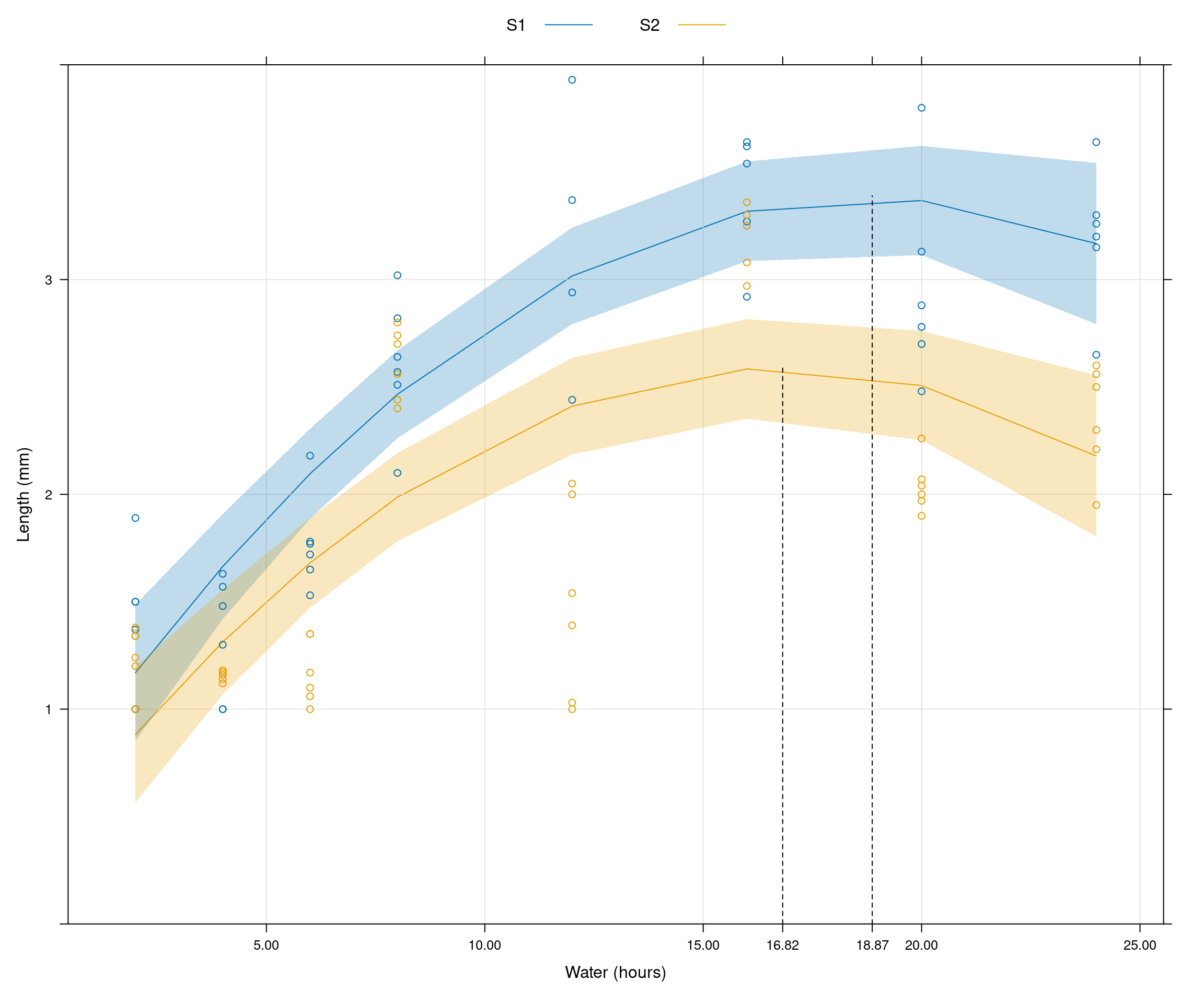
11.3 Multiple regression model with quantitative and qualitative variables
Example 11.3 Analysis of the growth of fungal hyphae.
The experiment was conducted to determine the effects of the duration of water exposure in a 24-hour period and temperature (degrees Celsius) in two different fungi.
Questions:
Do the two fungi being tested have the same growth pattern? Can I use the same model for both fungi?
water.time <- rep(c(4,8,12), each=9)

temperature <- rep(c(10,15,20,25,30,35,28), each=27)

fungi <- rep(c("S1","S2"), each=189)


fungi.l <- c(1.69,1.63,1.38,1.44,1.70,1.61,1.96,1.82,1.38,1.80,1.83,2.17,1.86,1.78,1.72,1.48,2.06,1.48,1.00,1.50,2.30,1.80,
             1.80,1.50,1.90,1.50,1.00,1.71,1.52,1.41,1.50,1.80,1.76,1.62,1.61,1.61,2.53,2.32,1.78,1.73,1.86,1.74,1.83,1.80,1.95,
                         1.76,1.96,1.33,2.18,1.90,2.01,2.20,2.45,2.23,2.00,1.82,2.05,1.79,2.07,1.29,2.25,1.70,1.71,3.95,4.18,4.46,4.36,3.78,
                         3.71,4.29,4.27,3.44,4.71,4.08,4.33,4.47,3.76,3.76,3.29,4.45,4.00,3.95,3.28,3.77,3.30,2.73,3.52,3.33,2.78,3.21,
                         3.22,4.14,5.67,5.13,5.33,4.32,4.43,3.73,4.56,3.77,3.70,3.13,4.00,4.71,2.91,4.00,5.09,3.89,2.84,2.84,2.06,2.75,2.75,
                         3.50,2.83,3.50,2.50,4.05,3.05,2.50,3.90,4.80,2.80,3.00,5.47,3.28,3.78,2.67,3.75,3.92,3.62,4.45,4.59,3.33,4.00,
                         1.00,2.27,1.00,2.27,1.00,2.27,1.00,2.27,1.64,3.79,1.25,3.79,1.25,3.79,1.25,3.79,1.25,2.52,2.64,1.00,2.64,1.00,
                         2.64,1.00,2.64,1.00,1.82,1.72,1.84,1.77,1.94,1.59,2.02,2.09,1.79,1.84,2.44,3.09,2.77,2.84,2.76,2.73,2.70,2.76,2.76,
                         2.02,1.42,2.02,1.47,2.30,2.50,3.01,3.70,2.89,1.29,1.40,1.50,1.29,1.33,1.63,1.83,1.00,1.00,1.50,1.70,1.52,1.45,
                         1.53,1.48,1.81,1.50,1.27,1.84,1.57,1.57,1.62,2.00,1.47,1.62,1.32,1.63,1.14,1.31,1.29,1.25,1.40,1.26,1.26,1.50,1.52,
                         1.30,1.31,1.13,1.32,1.38,1.77,1.50,1.79,1.77,1.67,2.06,1.94,1.39,1.33,1.41,1.61,1.56,1.52,1.84,1.50,1.83,1.80,
                         1.32,1.38,1.77,1.79,1.77,1.67,2.06,1.94,1.39,1.33,1.41,1.61,1.56,1.52,3.50,2.40,1.50,1.00,1.00,2.80,2.03,3.05,3.20,
                         2.14,1.95,2.11,2.12,2.17,1.92,1.51,2.21,2.23,2.56,2.70,2.74,2.40,2.44,2.80,1.91,2.89,2.53,2.59,2.24,1.77,2.62,
                         2.41,2.26,1.87,2.60,2.30,2.94,2.70,2.16,2.89,2.60,3.40,2.78,3.51,2.64,2.19,3.10,3.08,2.78,3.47,2.73,2.89,2.89,2.89,
                         3.11,2.64,2.97,2.45,2.61,3.15,3.10,2.35,2.38,1.70,1.38,1.50,1.89,1.58,1.86,1.27,1.41,1.64,1.54,1.84,1.69,2.02,
                         1.33,1.69,1.93,1.86,1.53,2.03,1.83,1.54,1.71,2.32,1.96,2.06,1.98,1.98,2.19,2.28,2.16,2.56,1.97,1.90,2.37,2.11,2.19,
                         2.17,2.34,2.08,3.10,2.12,2.17,2.39,2.74,2.55,2.62,2.31,2.48,2.19,2.48,2.00,2.85,2.93,2.48)


data <- data.frame(water=water.time,temp=temperature, fungi=fungi, resp=fungi.l)
head(data)
## water temp fungi resp
## 1 4 10 S1 1.69
## 2 4 10 S1 1.63
## 3 4 10 S1 1.38
## 4 4 10 S1 1.44
## 5 4 10 S1 1.70
## 6 4 10 S1 1.61library(lattice)
library(gridExtra)
p1 <- xyplot(resp ~ water, groups=fungi, data=data, type=c("a","p"), auto.key=list(space="top", columns=2))
p2 <- xyplot(resp ~ temp, groups=fungi, data=data, type=c("smooth","p"), auto.key=list(space="top", columns=2))
grid.arrange(p1,p2, ncol=2)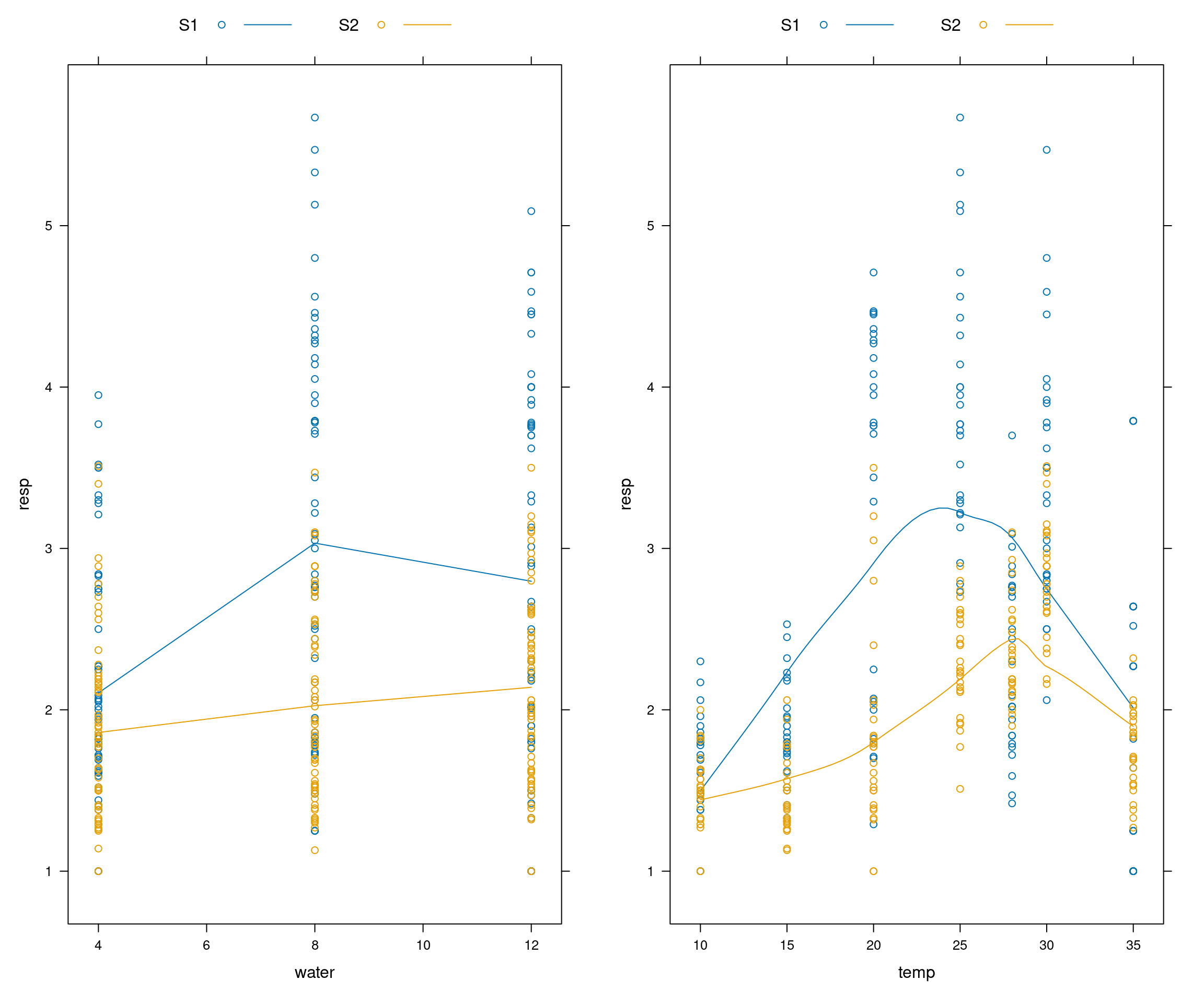
Model selection
library(MASS)

model.f <- lm(resp ~ fungi*water*temp + fungi*I(temp^2), data=data)
anova(model.f)
## Analysis of Variance Table
##
## Response: resp
## Df Sum Sq Mean Sq F value Pr(>F)
## fungi 1 38.305 38.305 79.1586 < 2.2e-16 ***
## water 1 14.882 14.882 30.7547 5.600e-08 ***
## temp 1 29.292 29.292 60.5323 7.377e-14 ***
## I(temp^2) 1 59.523 59.523 123.0054 < 2.2e-16 ***
## fungi:water 1 2.674 2.674 5.5265 0.01926 *
## fungi:temp 1 0.015 0.015 0.0305 0.86145
## water:temp 1 0.002 0.002 0.0041 0.94903
## fungi:I(temp^2) 1 13.953 13.953 28.8334 1.401e-07 ***
## fungi:water:temp 1 0.097 0.097 0.2003 0.65474
## Residuals 368 178.076 0.484
## ---
## Signif. codes: 0 '***' 0.001 '**' 0.01 '*' 0.05 '.' 0.1 ' ' 1model.s <- stepAIC(model.f)## Start: AIC=-264.51
## resp ~ fungi * water * temp + fungi * I(temp^2)
##
## Df Sum of Sq RSS AIC
## - fungi:water:temp 1 0.0969 178.17 -266.31
## <none> 178.08 -264.51
## - fungi:I(temp^2) 1 13.9525 192.03 -238.00
##
## Step: AIC=-266.31
## resp ~ fungi + water + temp + I(temp^2) + fungi:water + fungi:temp +
## water:temp + fungi:I(temp^2)
##
## Df Sum of Sq RSS AIC
## - water:temp 1 0.0020 178.18 -268.30
## <none> 178.17 -266.31
## - fungi:water 1 2.6743 180.85 -262.68
## - fungi:temp 1 13.4417 191.62 -240.82
## - fungi:I(temp^2) 1 13.9525 192.13 -239.81
##
## Step: AIC=-268.3
## resp ~ fungi + water + temp + I(temp^2) + fungi:water + fungi:temp +
## fungi:I(temp^2)
##
## Df Sum of Sq RSS AIC
## <none> 178.18 -268.30
## - fungi:water 1 2.6743 180.85 -264.67
## - fungi:temp 1 13.4417 191.62 -242.81
## - fungi:I(temp^2) 1 13.9525 192.13 -241.81anova(model.s)## Analysis of Variance Table
##
## Response: resp
## Df Sum Sq Mean Sq F value Pr(>F)
## fungi 1 38.305 38.305 79.5446 < 2.2e-16 ***
## water 1 14.882 14.882 30.9047 5.197e-08 ***
## temp 1 29.292 29.292 60.8275 6.412e-14 ***
## I(temp^2) 1 59.523 59.523 123.6053 < 2.2e-16 ***
## fungi:water 1 2.674 2.674 5.5535 0.01896 *
## fungi:temp 1 0.015 0.015 0.0307 0.86111
## fungi:I(temp^2) 1 13.953 13.953 28.9740 1.305e-07 ***
## Residuals 370 178.175 0.482
## ---
## Signif. codes: 0 '***' 0.001 '**' 0.01 '*' 0.05 '.' 0.1 ' ' 1summary(model.s)##
## Call:
## lm(formula = resp ~ fungi + water + temp + I(temp^2) + fungi:water +
## fungi:temp + fungi:I(temp^2), data = data)
##
## Residuals:
## Min 1Q Median 3Q Max
## -2.06998 -0.46676 -0.00033 0.42706 2.52498
##
## Coefficients:
## Estimate Std. Error t value Pr(>|t|)
## (Intercept) -3.0735480 0.4137920 -7.428 7.70e-13 ***
## fungiS2 2.5107835 0.5851902 4.291 2.28e-05 ***
## water 0.0865079 0.0154553 5.597 4.25e-08 ***
## temp 0.4743496 0.0382945 12.387 < 2e-16 ***
## I(temp^2) -0.0098933 0.0008479 -11.668 < 2e-16 ***
## fungiS2:water -0.0515079 0.0218571 -2.357 0.019 *
## fungiS2:temp -0.2861251 0.0541567 -5.283 2.17e-07 ***
## fungiS2:I(temp^2) 0.0064547 0.0011992 5.383 1.31e-07 ***
## ---
## Signif. codes: 0 '***' 0.001 '**' 0.01 '*' 0.05 '.' 0.1 ' ' 1
##
## Residual standard error: 0.6939 on 370 degrees of freedom
## Multiple R-squared: 0.471, Adjusted R-squared: 0.461
## F-statistic: 47.06 on 7 and 370 DF, p-value: < 2.2e-16The stepwise methodology using the AIC criteria for model selection presented the following models:
Fungi S1: \(E(y) = \beta_{0} + \beta_{1}X + \beta_{2}Z + \beta_{3}Z^{2}\)
Fungi S2: \(E(y) = \beta_{0} + \beta_{1}X + \beta_{2}Z + \beta_{3}Z^{2}\)
Equations
Fungi S1: $ -3.073 + 0.086X + 0.474Z - 0.009Z^{2}$
For fungi 2
\(\beta_{0}\) for S2 is \((Intercept) - fungiS2\) = \(-3.073 + 2.510 = -0.563\)
\(\beta_{1}\) for S2 is \(water - fungiS2:water\) = \(0.086-0.051=0.035\)
\(\beta_{2}\) for S2 is \(temp - fungiS2:temp\) = \(0.474-0.286=0.188\)
\(\beta_{3}\) for S2 is \(I(temp^2) - fungiS2:I(temp^2)\) = \(-0.009+0.006=-0.003\)
Fungi S2: \(-0.563 + 0.035X + 0.188Z - 0.003Z^{2}\)
Predictions
library(latticeExtra)
pred <- predict(model.s)
dat.graf <- data.frame(data, pred=pred)
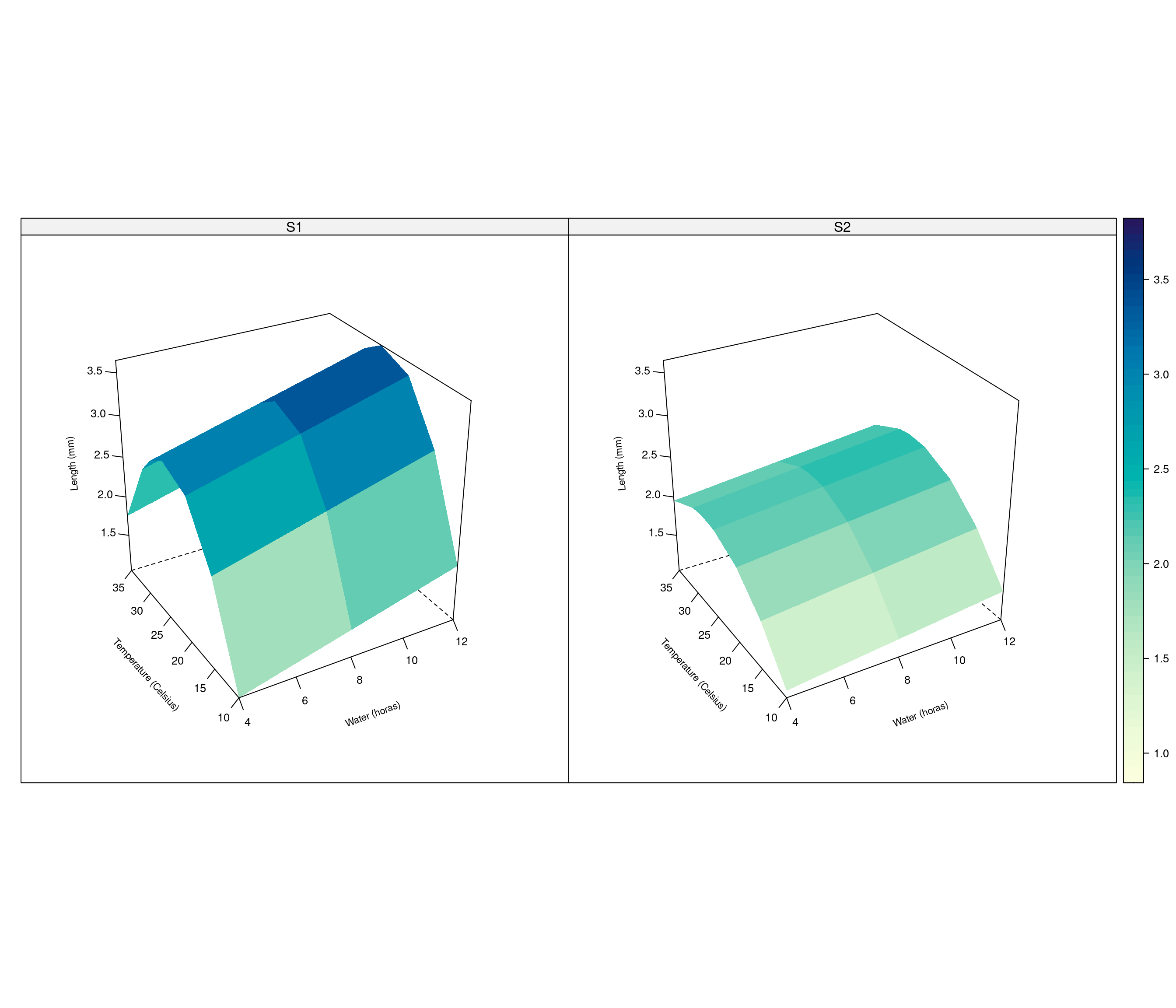
wireframe(pred ~ water + temp | fungi, data=dat.graf,
drape=TRUE, #colorkey=FALSE,par.settings = standard.theme(color = FALSE),
col='transparent',
scales = list(arrows = FALSE),
screen = list(z = 30, x = -60),
xlab=list("Water (horas)", rot=20, cex=0.7),
ylab=list("Temperature (Celsius)", rot=-48, cex=0.7),
zlab=list('Length (mm)', rot=95, cex=0.7),
par.box = list(col=c(1,1,NA,NA,1,NA,1,1,1)))