Chapter 11 Using climate models for climate scenarios

11.1 Definition climate scenario

A climate scenario is a plausible image of a future climate based on knowledge of the past climate and assumptions on future change (on increase of greenhouse gas (GHG) concentrations). They are constructed to estimate the impact of climate change. Usually they are constructed with the help of climate model information.

The terms “climate scenario” and “climate change scenario” are often used interchangeably. The term “climate change scenario” refers to a representation of the difference between the plausible future climate and the current or reference climate. A climate change scenario can be viewed as an interim step towards constructing a climate scenario.

The scenarios should not be treated as predictions of what will happen in the future, since they are based on assumptions on increases in GHG concentrations (plausible does not mean that the scenario is probable!).

11.1.1 Cascade of scenarios

A cascade of scenarios (based on uncertainties) has to be considered in developing climate and related scenarios for climate change impact, adaptation and mitigation assessment.

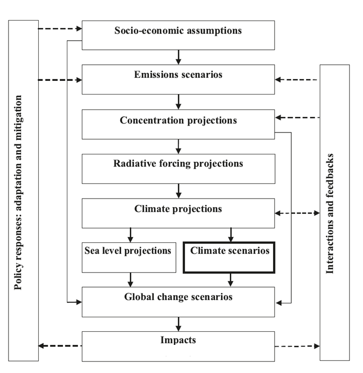
cascade

See also the UNFCCC webinar on approaches for developing climate scenarios (especially from minute 18:30)

11.2 Why do we use scenarios?

• By constructing scenarios based on different assumptions, we can quantify the impact of uncertainties about climate change. This can be uncertainties about the emissions of GHG, but also uncertainties about how the climate will react to an increase in GHG.
• Scenarios are plausible and consistent images of the future, based on our current knowledge of the climate system and about potential changes in GHG concentrations.
• Scenarios help us to understand climate change impacts and determine key vulnerabilities. They can also be used to evaluate adaptation strategies.

11.3 Constrution of IPCC scenarios

11.3.1 Types of scenarios

The Intergovernmental Panel on Climate Change - Task Group on Data and Scenario Support for Impact and Climate Assessment (IPCC-TGICA) classified climate scenarios into three main types (IPCC-TGICA, 2007), based on how they are constructed. These are:

• synthetic scenarios: particular climate elements are changed by a realistic arbitrary amount, for example, adjustment of temperature variable by +1, +2, and +3°C from a reference state, without the use of climate models.
• analogue scenarios: using a temporal analogue (using past climate record) or a spatial analogue to represent the possible future climate.
• climate model based scenarios: use outputs from Global Climate Models (GCM) or Regional Climate Models (RCM). They usually are constructed by adjusting a baseline climate (typically based on regional observations of climate over a reference period) by the absolute or proportional change between the simulated present and future climates.

The IPCC scenarios and the national climate scenarios that will be discussed later are all climate model based scenarios.

11.3.2 Steps in producing scenarios

The three main steps for developing IPCC climate change scenarios for the Fifth Assessment Report (AR5) in 2013 were:

• Developing emission scenarios and translating them to Representative Concentration Pathways (RCP) using Integrated Assessment Models (IAMs). The RCPs were designed in such a way that they represent a wide range of radiative forcing of the climate system at year 2100 and thus GreenHouse Gas (GHG) concentrations.
• Simulating the effect of different RCP’s on the climate with a large number of dynamical Earth System Models (ESMs).
• The IPCC climate scenarios are the difference of these projections compared to the reference climate, in the AR5 report the period 1986-2005 (mean changes per RCP are determined and the probable range).

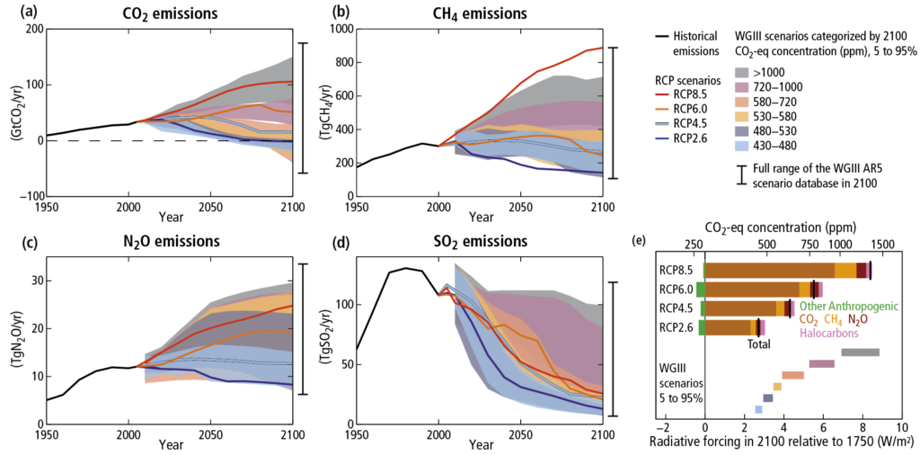
ipcc-scenarios

For several socio-economic development pathways the emissions of the various GHGs are determined (figures a-d).

Some GHGs have a stronger radiative forcing than others. The radiative forcing of all GHG’s is summed and expressed as the CO 2 -equivalent concentration (figure e; the CO 2 concentration that would give this radiative forcing).

The names of the RCP’s indicate the radiative forcing of each scenario around year 2100.

For IPCC especially the climate model runs from the Coupled Model Intercomparison Project (CMIP) are used. The range in model results for each RCP gives an indication of the uncertainties associated to the climate system reaction to the increase of GHG concentrations. Up to about year 2050 the ranges of the 4 RCP’s greatly overlap.

The mean change in global temperature (and other climate variables) over the results of the large number of climate model simulations for each RCP is calculated and compared to the reference period 1986-2005. The probable range covering about two-thirds of the range of the climate model simulations is represented by the bands around the thick lines.

11.4 National climate scenarios: why constructing them? and why are there differences?

National climate scenarios, in addition to the global IPCC climate scenarios, are developed in order to:

• Translate IPCC reports to the national scale: IPCC reports do not provide results for individual countries.
• Support the national climate adaptation policy, for which regional or local climate change information is needed.
• Provide a common framework for adaptation planning in different sectors of society.
• Support impact studies or develop adaptation options and strategies. With this information questions from various sectors in society can be answered. Moreover, national climate scenarios can be used for long-term planning of public and private sector organisations, to reduce exposure to climate risks and exploit potential new opportunities.
• Provide more relevant and appealing information on the national (or regional) scale in order to raise awareness.

11.4.1 Overview of national scenarios (January 2019)

Below links to national climate scenarios in various European countries (latest updated Jan. 2019). The timing for translating the global scenarios to national climate scenarios differs in each country. Methods used, the reference period, the time horizons, etc. may also differ.

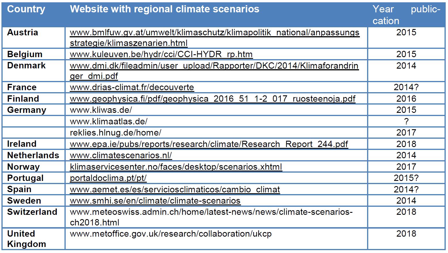
national-scenarios

Source: updated from Bessembinder et al., 2018

11.4.2 Reasons for differences between national scenarios

National climate scenarios of European countries differ in many aspects. Although they generally use the global climate models adopted in the IPCC reports, they also use results form large European projects on climate modelling for which downscaling of results from GCMs is done with RCMs, for example PRUDENCE, ENSEMBLES, EUROCORDEX.

Factors

Which global and regional climate models are used, reference period, RCPs, time horizons, climate variables are included may depend on the availability and accessibility of the climate model output in a country. Moreover, the climate models that the organisation(s) developing the national/regional climate scenarios can run, the purpose of the development of climate scenarios, the relevant areas for the country/region and the sectors included may also influence the way national climate scenarios are developed.

11.4.3 Examples of differences between national scenarios

Some differences between the national climate scenarios in some European countries (for the scenarios per country mentioned in the table on slide 16).:

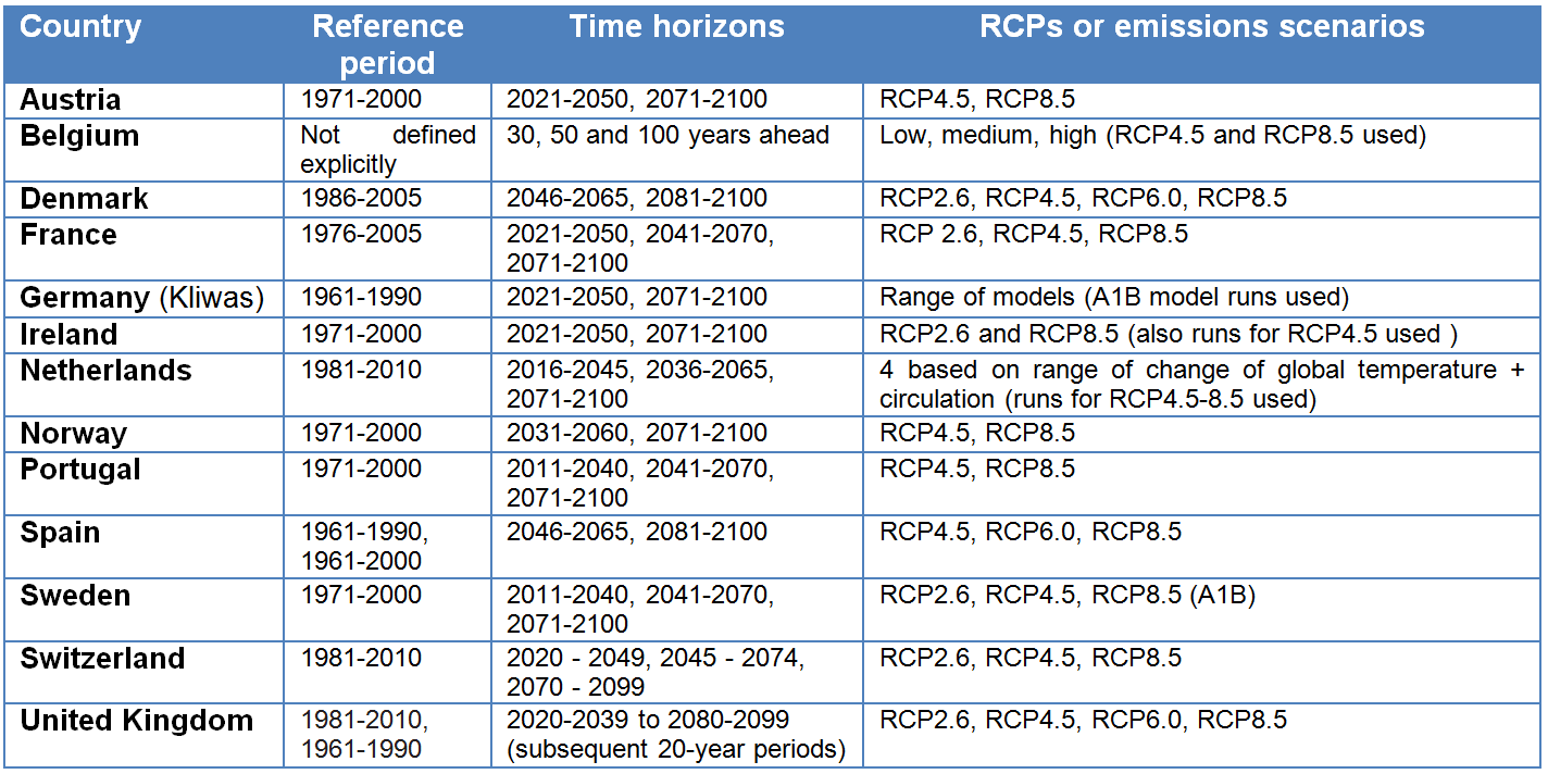
differences-scenarios

Source: updated from Bessembinder et al., 2018

11.4.4 RCPs used in national scenarios

Although there are 4 RCPs they are not always used for the construction of national/regional climate scenarios. In almost all cases of the table in the previous slide RCP8.5 and RCP4.5 were used.

• RCP8.5 represents the highest emissions and consequently the largest change in climate (it was often refered to as business-as-usual or worst-case).
• RCP4.5 is often used to indicate the lower probable climate change. Although RCP2.6 is possible, it is not considered very likely. Moreover, there are also less climate model runs with RCP2.6.
• In some scenarios RCP2.6 is used to construct the climate scenario with the lowest climate change and RCP8.5 for the higest climate change, leaving out the others.
• RCP6.0 is not used much in the scenarios as it does not necessarily add much additional information when showing the range of possible climate change.

In older national climate scenarios, the SRES (Special Report on Emission Scenarios) emission scenarios may still be used.

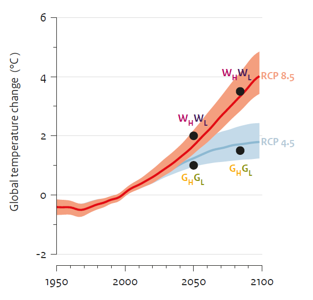
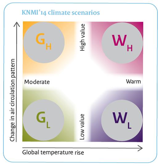
Example: national scenario of the Netherlands

In the figure below the selection of climate scenarios is based on information from RCP8.5 and RCP4.5. RCP8.5 represents high levels of climate change when few mitigation measurements are taken, and RCP4.5 low levels of climate change when many mitigation measurements are taken. RCP2.6 was considered less relevant.

netherlands2

netherlands1

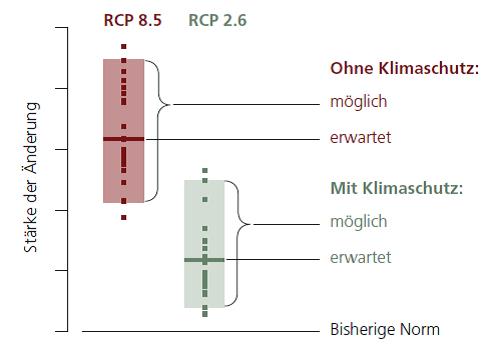
Example: national scenario of Switzerland

Range of climate change (“Starke der Anderung”) in the CH2018 climate scenarios for Switzeland compared to what is currently used to describe the climate (“Bisherige Norm”). For RCP8.5 and RCP2.6 the mean change in an ensemble of EUROCORDEX models is shown (“erwartet”) and the possible range (“moglich”) (Source: CH2018, 2018)

In the figure below shows the Swiss CH2018 climate scenarios RCP8.5 and RCP2.6 used to describe the range of levels of climate change for the future. RCP8.5 represents high levels of climate change when few mitigation measures are taken (“Ohne Klimaschutz”), and RCP2.6 represents what the levels of climate change may look like when many mitigation measures are taken (“Mit Klimaschutz”). The RCPs selection for the Swiss case differs from that in the Netherlands.

switzerland

11.4.5 Selection of reference period

Diverse criteria drive the selection of the reference period:

• Same reference period as the former national climate scenarios to make comparison easier.
• Two reference periods may be used: a recent period (e.g. 1981-2010) and a previous climate scenarios (e.g. 1961-1990) reference period. This makes comparison with earlier scenarios easier.
• Same reference period as that used in IPCC to make comparison with IPCC easier.
• Same reference period used for the “climate normals” (to describe whether the weather is above or below normal). The availability of the description of these normals (and the ranges) makes it easier to understand what will be the future climate.
• Most recent period of 30 years, since that comes closest to what society will consider the “current climate”.

In most cases a period of 30 years is used as reference period. However, since there maybe a considerable trend in climate in 30 years, a period of 20 years may be used as reference. For example IPCC used 1986-2005 as reference period in the Fifth assessment report.

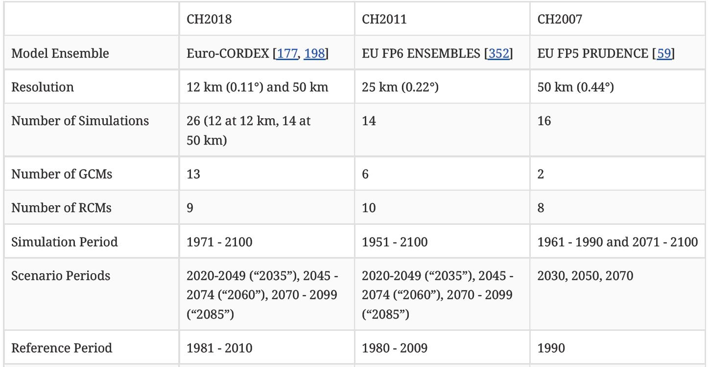
Example selection of reference period (Switzerland):

The table below shows that the reference period (last row) used in Switzerland has changed somewhat with the various sets of climate scenarios publised in 2007, 2011 and 2018. For the CH2018 scenarios the most recent “normal period” 1981-2010 is used. This dataset may have not been available in 2011 therefore, the most recent 30 year period 1980-2009 was used in CH2011. For the CH2007 scenarios, “1990” is mentioned as reference (probably meaning the 30 year period around this year, 1976-2005). This shows that criteria to choose a reference period selection may change over time.

switzerland-reference

Source: CH2018, 2018

11.4.6 Selection of time horizon

The selection of the future time horizons greatly differs for each country:

• In most cases a time horizon around the middle of this century is chosen, as well as a time horizon at the end of the 21st century.
• In some countries a “near-future” time horizon is also used, for example 2021-2050. The change in this period, compared with the reference period is often not significant and differences between scenarios are often not significant.
• Most countries use 30 year time slices but 20 year time slices are not uncommon. A 30 year period is commonly used to describe the climate. However, since a 30 year period can contain clear trends, especially for temperature, 20 year time slices are also used regularly nowadays.

Example of time horizon selection: the Netherlands & Switzerland

In the figures below year 2050 (2036-2065) and 2085 (2071-2100) are chosen as time horizons for the KNMI14 scenarios in the Netherlands. In Switzerland the time horizons 2035 (2020-2049), 2060 (2035-2074) and 2085 (2070-2099) for the CH2018 scenarios are used.

Average summer temperature in the Bilt, Netherlands: observations (three 30-year averages in blue), KNMI’14 scenarios (2050 and 2085, in four colours) and natural variations (in grey, for 30-year averages; Source: KNMI, 2015)

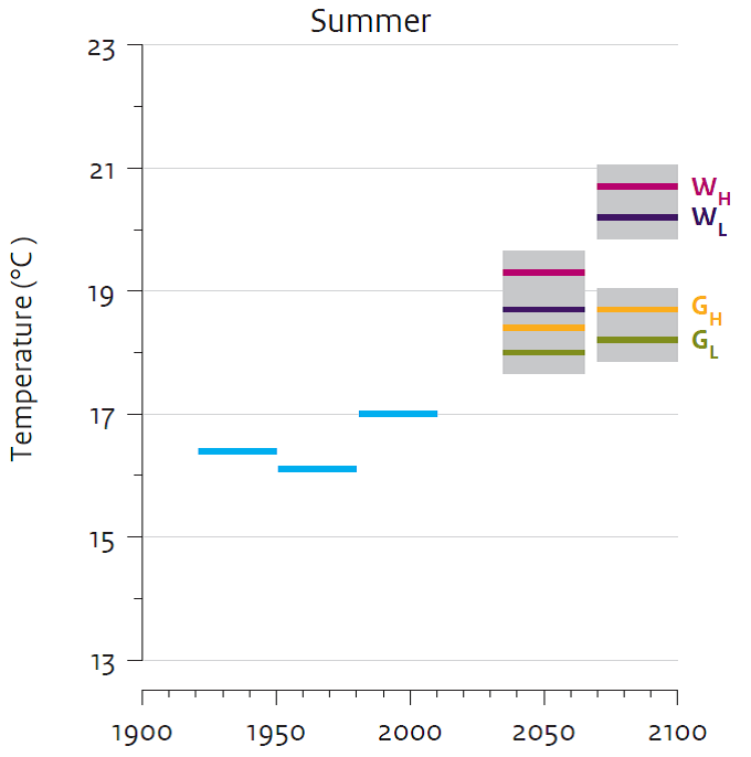
horizon-netherlands

The reference period and time horizons used in the CH2018 climate scenarios for Switzerland (Source: CH2018, 2018)

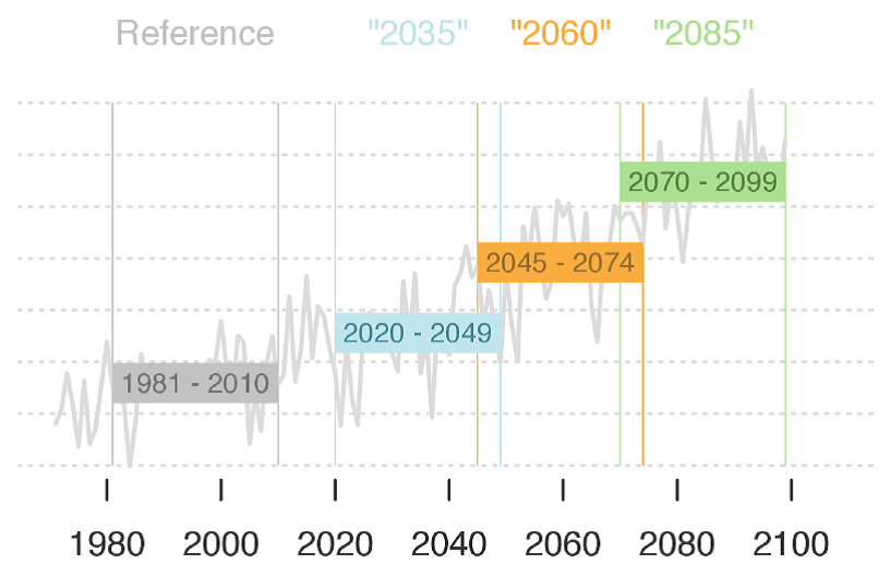
horizon-switzerland

11.4.7 Selection of global climate models (GCMs)

Often during the development of national (or regional) climate scenarios the most recent GCMs (or the more sophisticated Earth System Models) are first analysed to discover the range of change they show for, among others, temperature and precipitation. Various approaches can be used:

• Use all: use the majority of available GCMs and leave out only the models that perform the worst for the country of interest. In practice this means that the majority of GCMs used in the IPCC reports or the CMIP projects are taken into account. Hardly any of these models perform poorly for all climate variables for the country of interest.
• Only use the best: only select the GCMs that perform the best for the region or country of interest, i.e. the climate models that simulate better the current climate and past trends (small bias, correct amplitude of temperature and precipitation throughout the year, good air circulation patterns, etc.).

The choice of climate models is also partly determined by the ease and availability of data (CMIP5 data are available through the Climate Data Store). For further downscaling a selection of RCMs may be used.

Example of selection of climate models: the Netherlands

For the development of the KNMI14 climate scenarios (Netherlands) a large range of GCMs (and RCPs) was used to determine the range of potential global temperature change and the related local temperature range in the Netherlands. In the former KNMI06 climate scenarios only the best performing GCMs for air circulation were used (however, this covered more or less the range of all available GCMs).

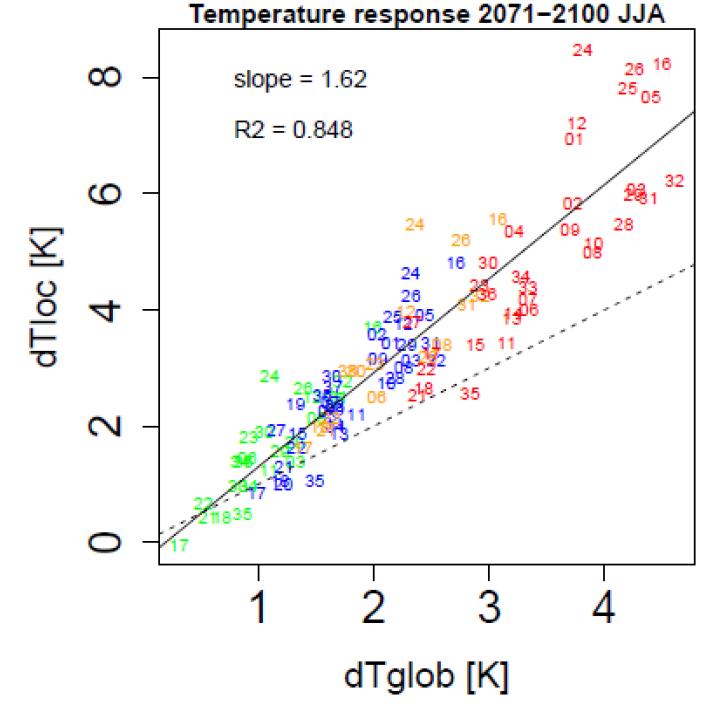
netherlands-gcm

Figure: Temperature change in the Rhine basin (dTloc) per GCM/RCP combination in 2071-2100 relative to 1976-2005 as function of global temperature change (dTglob). Numbers= GCMs; green=RCP2.6, blue=RCP4.5, orange=RCP6.0, red=RCP8.5; dotted line 1:1. (Source: KNMI, 2014)

Example of selection of climate models: Switzerland

For the development of the CH2018 climate scenarios (Switzerland), the range of seasonal temperature change in the used CORDEX-GCMs and CORDEX-RCMs was compared with the range in temperature change for the IPCC AR5 GCM’s for Switzerland. Although the used GCM’s (CORDEX) do not always cover the same range as the IPCC GCMs, the chosen RCMs cover most of the range presented by the IPCC GCMs.

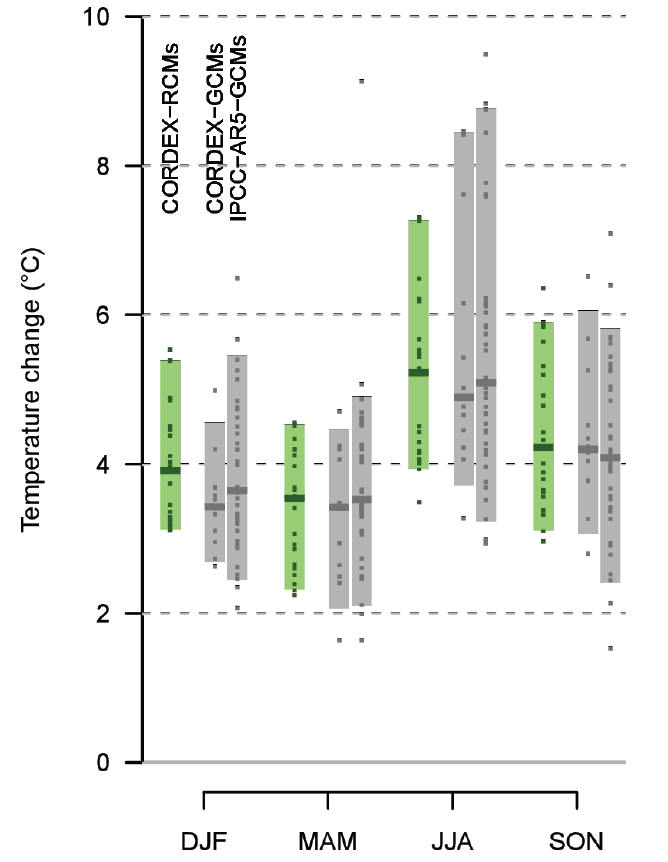
switzerland-gcm

Figure: Temperature change per season for Switzerland around 2085 and RCP8.5, based on various model ensembles. Quantile-based uncertainty ranges (colored bars 5-95%) and individual models (points) are shown. Green bars=CORDEX RCMs, left grey bars=CORDEX-GCMs, right grey bars=IPCC-AR5-GCMs (Source: CH2018, 2018)

Example selection of Global Climate Models

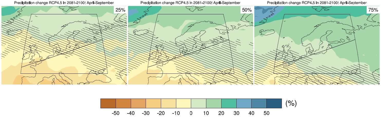
Climate scenarios generally aim to show the possible range of changes in the future or a large part of this range. Therefore, looking at the range of changes in an ensemble of GCMs is a useful first step. If certain GCMs show a decrease in seasonal precipitation and others show an increase in annual precipitation, it may be good to have this expressed in the national climate scenarios. The figures below show the percentiles in such an ensemble. They show that for the UK and Netherlands some GCMs have an increase (75% percentile) and others a decrease of precipitation in the summer half year (50% and 25% percentiles).

selection-global-gcm

Figure: Change in precipitation sum in 2081-2100 in April-September relative to 1986-2005 for North and Central Europe. Middle: average of the GCM ensemble, left 25% percentile, right: 75% percentile. Hatching: 20-year mean differences less than the standard deviation of model-estimated present-day natural variability (Source: IPCC AR5 (2013) WG1 Annex1)

11.4.8 Selection of RCMs for downscaling

Although there are several methods for downscaling (statistical and dynamical) often dynamical downscaling with the help of RCMs is used. These models help to get a more detailed view on the effects of global climate change for a country and its regional differences. Either an ensemble of RCMs is used to construct the national climate scenarios or one RCM is used to downscale the changes represented by various GCMs.

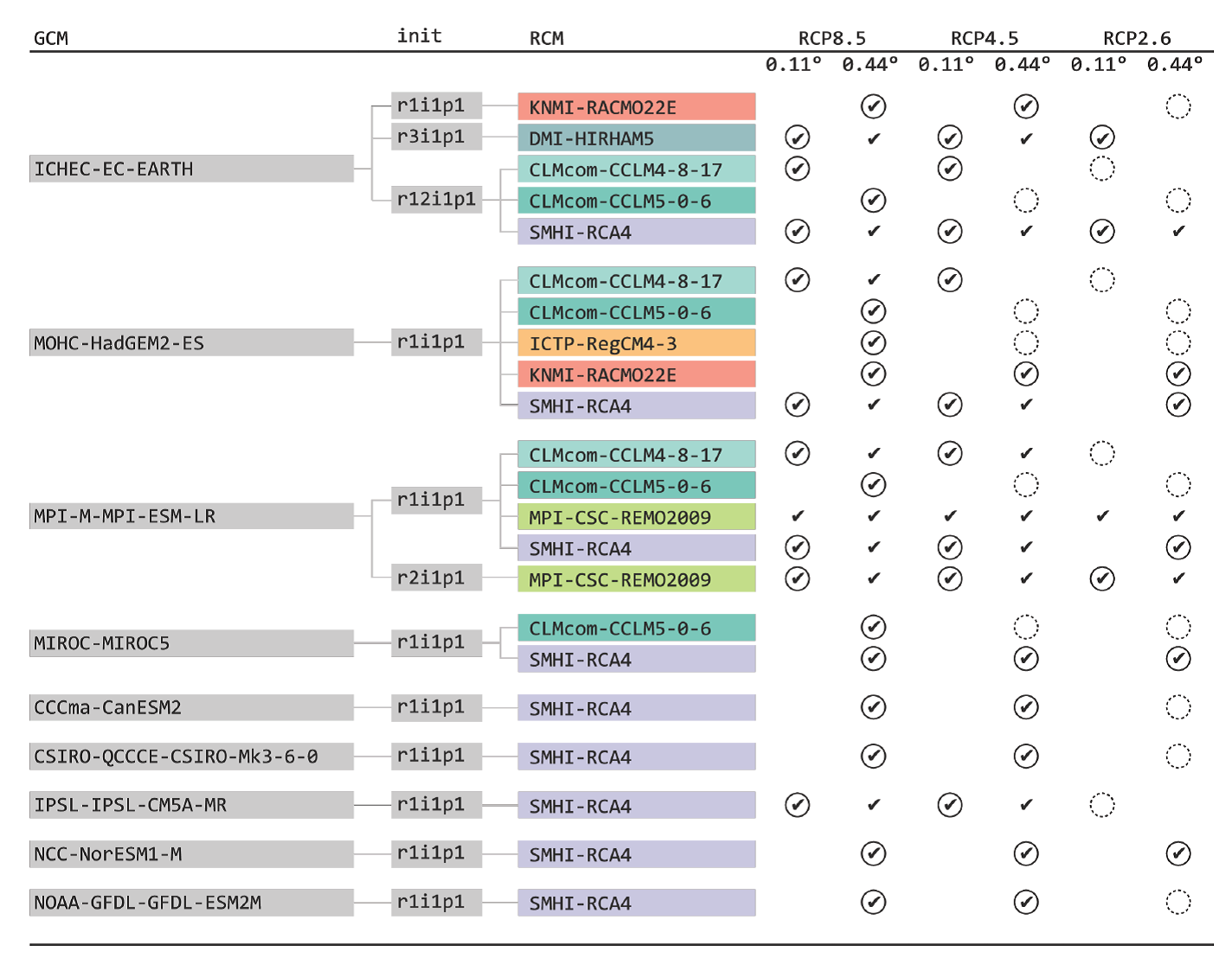
In Switzerland the ensemble of EURO-CORDEX RCMs is used (see table:various GCM-RCM combinations), whereas in the Netherlands an ensemble of various runs with the GCM-RCM combination EC-Earth (GCM) and RACMO (RCM) was used for downscaling.

euro-cordex-runs

Figure: EURO-CORDEX runs used for CH2018 climate scenarios. Checkmarks indicate existing simulations, circles mark the simulations used for multi-model combination, and empty dashed circles show the simulations substituted by pattern scaling (source: CH2018, 2018)

11.4.9 Approaches to use ensembles of climate models

Different approaches can be used to construct climate scenarios:

• From the ensemble of available climate models, individual model runs can be chosen to represent one scenario (for various time horizons), e.g. for high and for low emissions. Often they are chosen so that they span a considerable part of the uncertainty in the ensemble.
• On the basis of the ensemble of climate model runs for all used RCPs the mean change in all model runs is calculated together with specific percentiles (e.g. 25% and 75%). The percentiles are than considered scenarios. Often such percentiles are interpreted as probabilities however, they only give an indication on how often a certain change is observed in the ensemble used.
• The mean change of the ensemble of model runs for each RCP is calculated together with specific percentiles (e.g. 25% and 75%). In this way “probabilistic” estimates of climate change per RCP are constructed.

Example of climate model construction: UK and Switzerland

Probabilistic estimates of climate change for each RCP are constructed for both the UKCP18 (UK) and CH2018 (Switzerland) climate scenarios.

temperature-change-0

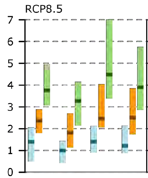
Figure: Range (5-95%) of air temperature change per season compared to 1981-2010 for RCP8.5 for around 2035 (blue), 2060 (orange) and 2085 (green) for the northwestern part of Switzerland (Source: CH2018, 2018)

temperature-change

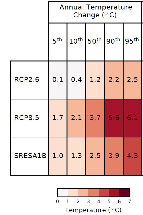
Figure: Projected change in temperature for the UK region per RCP or SRES scenario from 1981-2000 to 2080-2099 using the probabilistic projections (Source: UKCP18, 2018)

11.4.10 Level of detail in climate scenarios

The level of details and amount of information in the national climate scenarios in the various European countries differ considerably. In some countries only the information on annual or seasonal average changes in temperature and precipitation is presented. In other countries information is presented for a large number of climate variables also including extremes. In general, more detailed information is given in countries where there is a strong interaction with users and where climate scenarios are used to estimate the impact of climate change on several sectors.

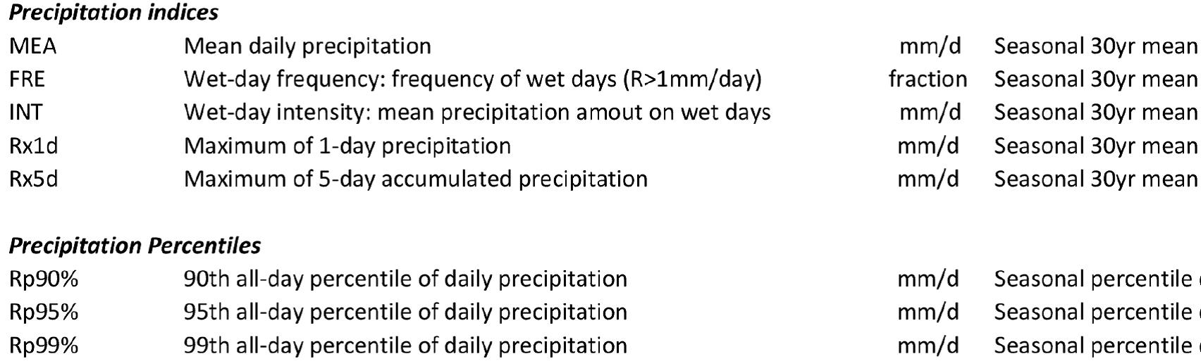
detail-level

Figure: Example of precipitation indices that are calculated for the Swiss CH2018 climate scenarios (Source: CH2018, 2018)

11.4.11 Additional information delivered with the climate scenarios

In some countries the national climate scenarios consist of a table with changes relative to each climate scenario. In other countries additional information is provided to help users to carry out further impact studies. For example daily time series, representative of the various climate scenarios for certain time horizons, can be provided. These time series are often obtained with the help of the underlying climate model runs for the climate scenarios, although different methods may be used to generate this information (statistical downscaling, bias correction, delta methods).

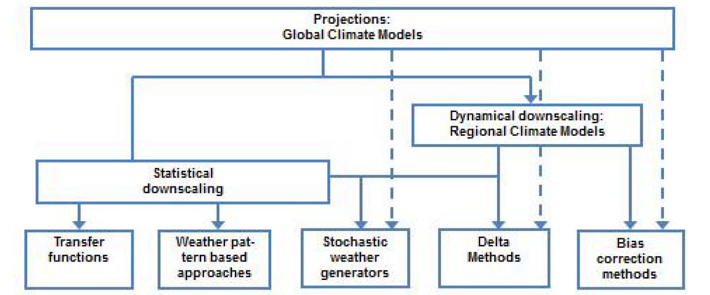
additional-data

Figure: Downscaling and bias removal methods (Source: Bessembinder, 2015)

Example: Switzerland

In Switzerland additional high resolution gridded datasets are provided in addition to presenting the changes in various climate variables for various time horizons and RCPs. The figure below shows information on the current and future climate at various weather stations, as well as high resolution gridded datasets for further impact studies. Here Quantile Mapping (QM, bias-correction method) is used to provide the additional information:

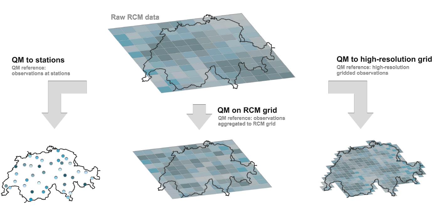
quantile-mapping

Figure: Quantile mapping methods and related data products. All variants produced for the entire CH2018 RCM ensemble but for different sets of meteorological variables (Source: CH2018, 2018)

11.4.12 Consistency between climate variables

Depending on the method used, the changes in various climate variables may show more or less consistency. For further impact analysis consistency among climate variables is often important, since the impact is determined by various climate variables.

• Climate scenarios that are based on individual climate model runs will show consistency between the various climate variables, since the climate models have internal consistency (note that statistical downscaling or bias-correction methods may affect the consistency somewhat).
• An ensemble of climate model runs may show a range of change in for example summer precipitation and summer temperature. The highest increase for summer temperature likely does not occur at the same time as the highest increase for summer precipitation.

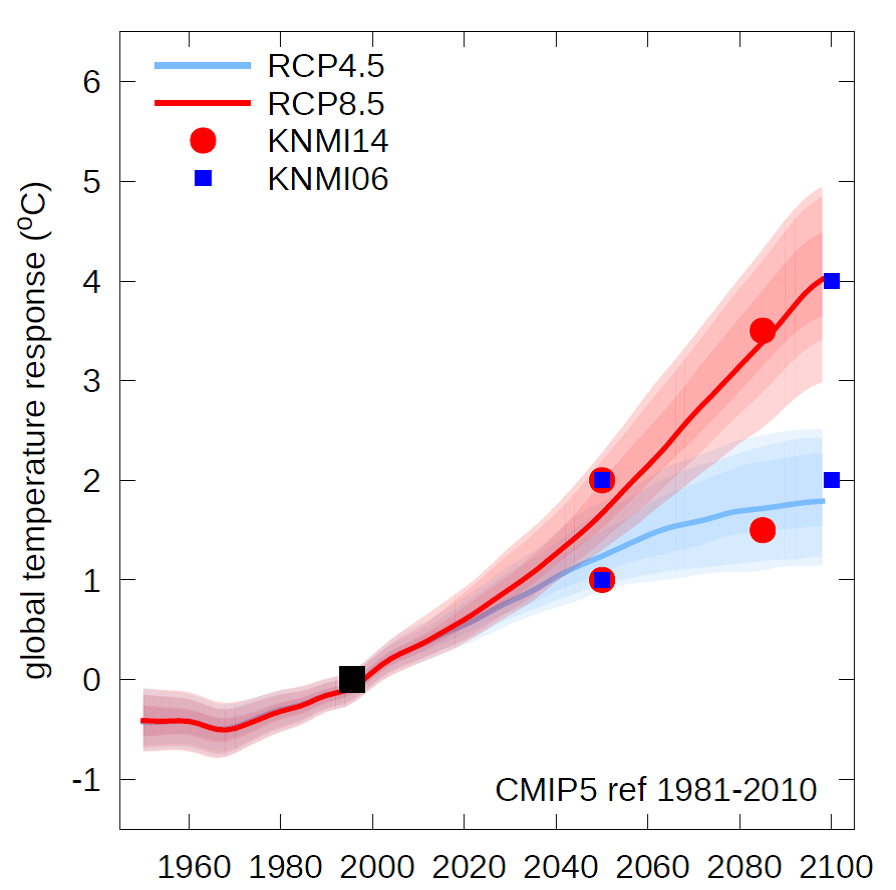
11.4.13 Representation of uncertainties

• Model uncertainty is represented by the spread of climate model output for each RCP. Some countries use the mean change per RCP (no model uncertainty), whereas others show also extreme percentiles for each RCP. The more climate models are used, the more the model uncertainty is represented. The more extreme the percentiles (e.g. 5-95%) the more of the model uncertainty is represented. Up to 2050, model uncertainty is relatively the most important uncertainty (see figure).
• Natural or internal variability: Not all countries present information on natural variability.
• Scenario uncertainty is represented by the differences between the RCPs means. Countries may differ in the RCP’s they use for the development of their national climate scenarios. Countries that use RCP8.5 and RCP2.6 present the largest part of the scenario uncertainty. This uncertainty is especially important in the second half of the 21st century (see figure).

How much of the various sources of uncertainties is presented in the national climate scenarios varies for each country (for types of uncertainties see the dedicated chapter on uncertainties.

Example of uncertainty representation: the Netherlands & Switzerland

uncertainty-netherlands

Figure: In the KNMI14 climate scenarios the temperature of the IPCC 10-90% range for the RCP8.5-RCP4.5 is used instead of the mean of the RCPs. In this way both scenario and model uncertainty are taken into account. This is especially important for the period up to 2050, which is of most relevance to users.

uncertainty-switzerland

Figure: Range (5-95% of the EURO-CORDEX models used) of air temperature change for each season compared to 1981-2010 for RCP8.5. Around 2035 (blue), 2060 (orange) and 2085 (green) for the northwestern part of Switzerland (Source: CH2018, 2018). Source: KNMI, 2014

Examples of natural variability representation: the Netherlands and the UK:

natural-variability-netherlands

Figure: Change of average summer temperature in the Netherlands in the KNMI’14 climate scenarios. The grey bands represent the 30-year natural variability based on the variability in the current climate (Source: KNMI, 2015).

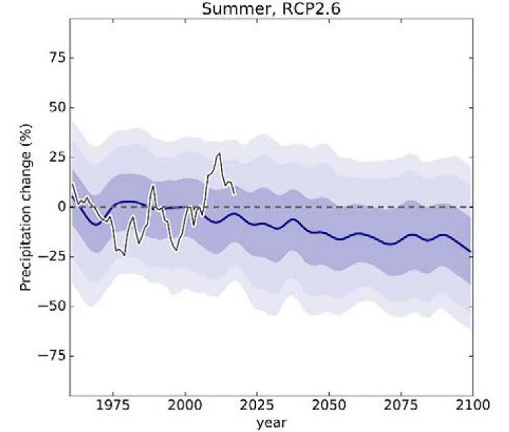
natural-variability-uk

Figure: Change of average summer precipitation in the UK under the RCP2.6 in the UKCP18 climate scenarios. The bands around the thick line represent various percentiles for the year to yearnatural variability for the past and future climate (Source: UKCP, 2018).

11.5 References