Chapter 3 Data Resources Introduction

3.1 What are essential Climate Variables?

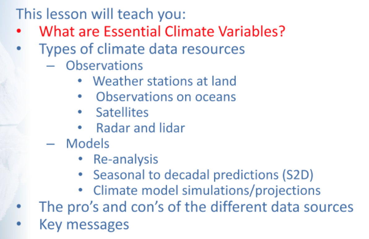
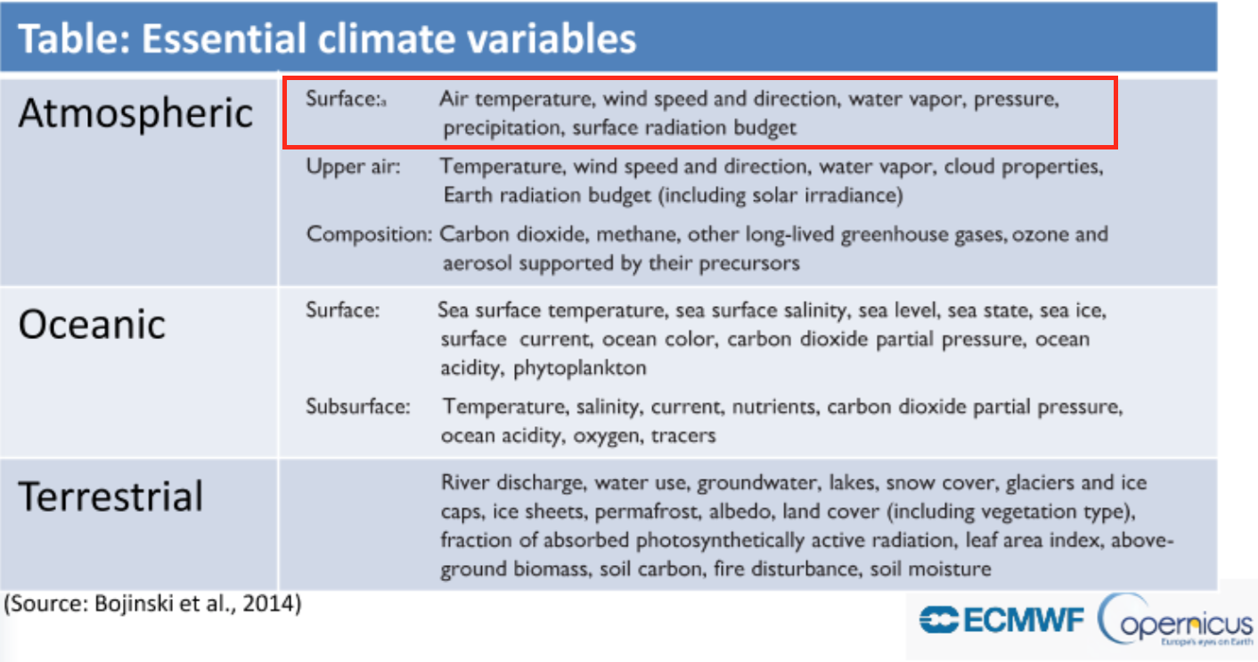
The Global Climate Observing System (GCOS) has developed 50 measurable Earth System Parameters : the Essential Climate Variables (ECVs). ECV = physical, chemical or biological variable or a group of linked variables that critically contribute to the characterization of Earth’s climate. ECVs are selected based on relevance, feasibility and cost effectiveness. See below figure for all ECVs: atmospheric (surface, upper air and composition), oceanic (surface and subsurface) and terrestrial. This lesson will focus mainly on atmospheric surface climate variables, as they are most often used in (sectorial) impact studies:

• Air temperature
• Wind speed and direction
• Water vapour
• Pressure
• Precipitation
• Surface radiation budget

3.2 Types of climate data resources

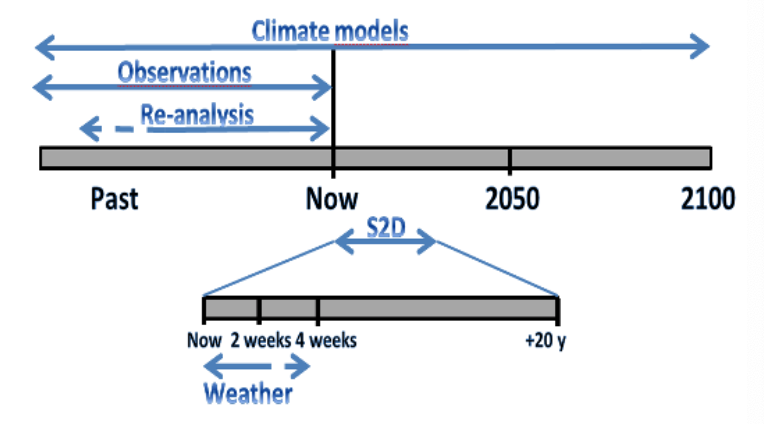
Various data sources can be used, categorised based on the period (past - future) and timescale (weeks, years) for which they provide data:

3.2.1 Observations

Observations ony provide information on the past and current climate. Besides the traditional observation stations on land there are many more direct and indirect observation methods:

3.2.1.1 DIRECT (in-situ) observations

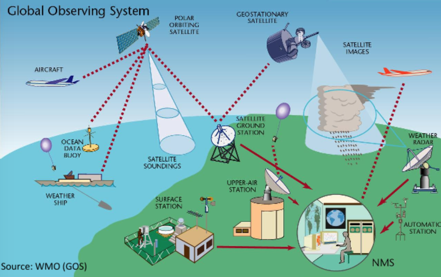
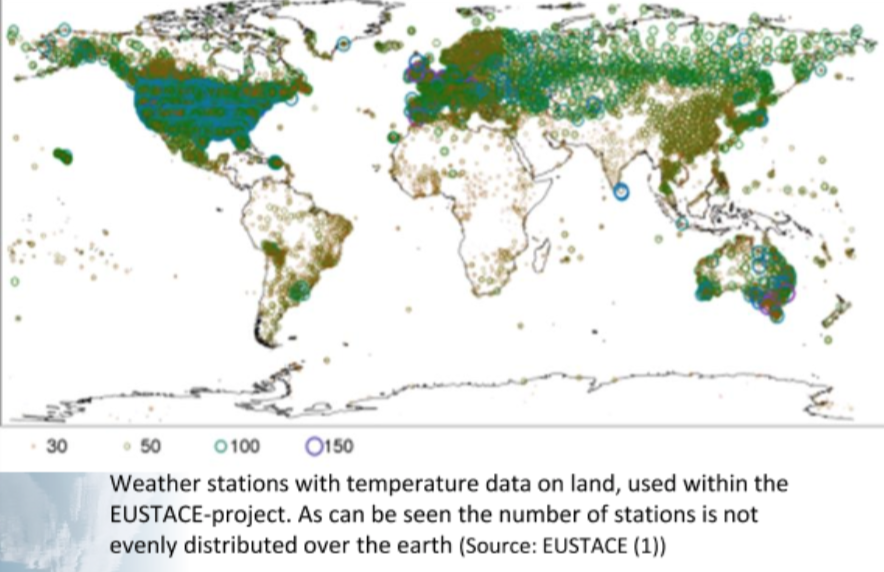
• Weather stations: there are thousands of weather or meteorological stations measuring at or near the Earth’s surface meteorological parameters such as atmospheric pressure, wind speed and direction, air temperature and relative humidity. These are observations at one location, or “in situ”. The number of stations is not evenly distributed over the Earth (see figure below). The WMO formulated standards for these stations (eg: T measured at 2 m height, no high vegetation around the station, …). For more info see WMO - best practices.

  

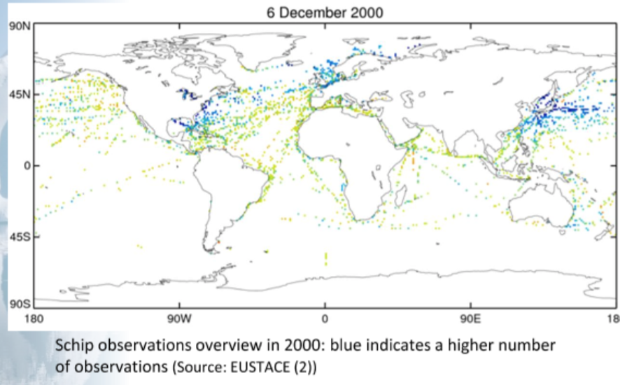
• Over the oceans the Global Observing System (GOS) relies - in addition to satellites - on ships, moored and drifted buoys and stationary platforms. The number of observing ships is around 4000, 1000 of them report observations every day.

  

3.2.1.2 INDIRECT Observations

As there are no records of climate from direct measurements before the 1600s, other sources are used to estimate and investigate the climate further back in time:

• Tree-rings and ice-cores: used to infer changes in temperature and precipitation
• Depth profiles of temperature in oil-drilling boreholes can be used to estimate the changes in air temperature over recent centuries
• Corals can be used to estimate oceanic temperature and sea-level changes

None of these indirect, or ‘proxy’ methods are as precise as direct instrumental measurements. Also, there are few proxy datasets, so it is very difficult to obtain reliable estimates of past global temperatures. However, long-term temperature trends derived from borehole and other independent proxy data are in reasonable agreement, confirming the climate in the past two thousand years, was not as warm as it has been in recent decades.

3.2.1.2.1 Satellites

Satellites are normally equipped with visible and infra-red imagers and sounders from which one can derive many meteorological parametres. Several over the polar-orbiting satellites are equipped with sounder instruments that can provide vertical profiles of temperature and humidity in the atmosphere in cloud-free areas. Geostationary satellites can be used to measure e.g. wind velocity in the tropics by tracking clouds and water vapour. Recent developments have made it possible to derive temperature and humidity information directly from satellite information.

Gridded observation products available at C3S

Types of satellites:

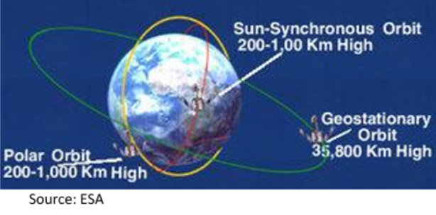
• Geostationary satellite: earth-orbiting satellite placed at an altitude of around 35800 km directly over the equator, that revolves in the same direction the earth rotates (west to east), and therefore constantly observes the same path of the earth.
• Polar orbiting satellite: closely parallels the earth’s meridian lines, thus having a highly inclined orbit close to 90°. It passes over the north and south poles each round. As the earth rotates to the east beneath the satellite, each pass monitors and area to the west of the previous pass. These strips can be pieced together to produce a picture of a larger area.

3.2.1.2.2 Radar and Lidar

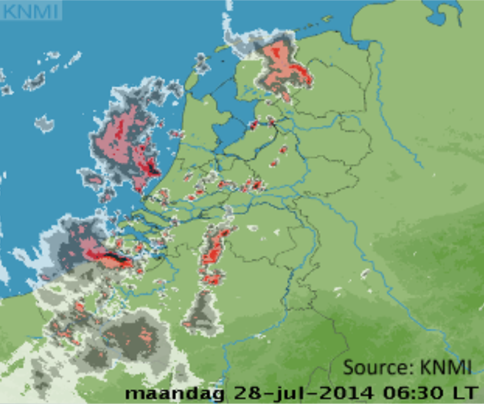
Weather radars have been used in the detection of precipitation rates since the 1950s. The first figure below shows and example of a rainfall radar image. In principle the method is based on sending out a radar pulse and measuring the return signal. The signal has to be translated into a precipitation rate with the help of in situ measurements (see second figure).

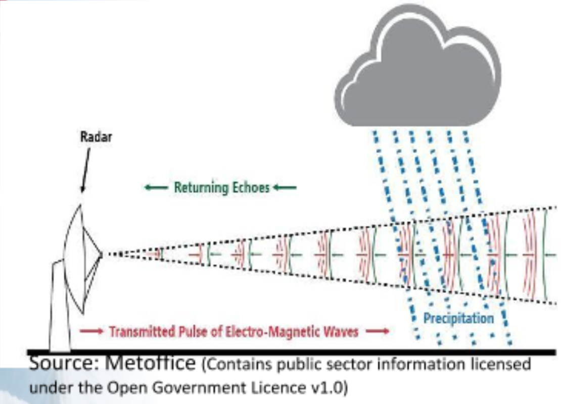
Dual polalized or doppler radars can measure wind and rainfall. They enable more accurate determination of precipitation types and sizes. This makes it easier to see whether the precipitation consists only of rain or also contains snow or hail (see video explanation).

Instead of using a radar pulse, Lidar (Light Detection And Ranging) is using laser light to study atmospheric properties from the ground up to the top of the atmosphere. Such instruments have been used to study, among others, atmospheric gases, aerosols, clouds, wind and temperature.

3.2.2 Models

For more information about model selection, see the dedicated chapter below

A climate model is a numerical representation of the climate system based on physical, chemical and biological properties of its components, its interactions and feedback processes.

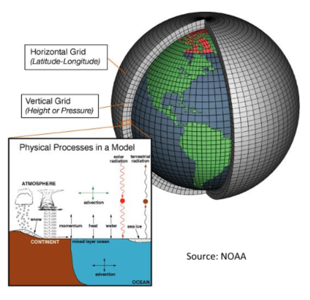
Climate models are systems of differential equations based on the basic laws of physics, fluid motion and chemistry. To “run” a model, scientists divide the planet into a 3-dimensional grid, apply the basic equations, and evaluate the results. The models calculate winds, heat transfer, radiation, relative humidity, and surface hydrology within each grid and evaluate interactions with neighboring points (IPCC, 2007). See also video explanation from the UK MetOffice and an introduction to climate modeling from Climate Literacy.

3.2.2.0.1 Difference between weather and climate models

• Weather consists of the short-term (minutes to months) changes in the atmosphere. Weather is described in terms of temperature, humidity, precipitation, cloudiness, brightness, visibility, wind, and atmospheric pressure, as in high and low pressure. In most places weather changes from minute-to-minute, hour-to-hour, day-to-day, and season-to-season. Weather is predictable up to about 2 weeks ahead in the mid-latitudes and in the tropics somewhat longer.
• Climate is the description of the long-term pattern of weather in a particular area. Climate is the average weather for a particular region and time period, and the probability of extremes. Usually a period of 30 years is used to describe the climate. Examples of described climate variables are precipitation, temperature, humidity, sunshine, wind velocity, phenomena such as fog, frost and hail storms. Also vegetation changes, changes in glaciers/icecaps etc. can be described.

Weather and climate models both follow the basic laws of physics, fluid motion and chemistry. However, they differ in some aspects:

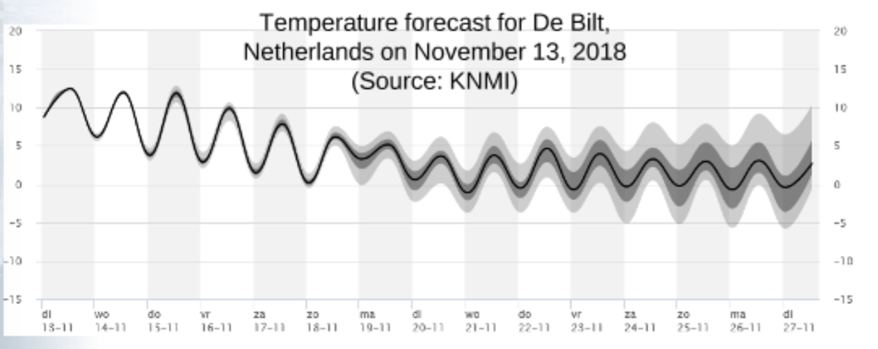
• Weather model: predicts in most cases til about 15 days into the future, while a climate model can integrate forward in time for hundreds of years. In a weather model, we care about when and where a storm or front occurs. In a climate model we care about the statistics (averages and probabilities of extremes). Since the weather of tomorrow depends strongly on the weather of today, the initial conditions for the simualtion of the weather are very important (initial value problem)
  • Model-based weather forecasts are generally less reliable beyond a week, because the atmosphere is an inherently chaotic system. Small changes in observed conditions, which are fed to the model regularly, can produce completely different weather forecasts a week into the future, because the atmosphere is very dynamic.
• In climate models you get climate variables for each day, but you don’t really care on which day and exact location you get a certain value for this variable as long as the long term statistics are correct for this location. This does not depend on the initial conditions of the simulation, but it depends on the parameters in the model itself (boundary value problem).
  • Climate models aren’t trying to predict what is going to happen at a specific place and point in time. They cannot produce a forecast for, say, the 15th of March 2077, or even not for tomorrow! Instead, climate models are used to determine how the average and extreme conditions will change. Will it be on average warmer or cooler, wetter or drier, in England over the next 50 years? This is information we need if we’re going to construct e.g. bridges or the water management system for the next decades.

3.2.2.1 Re-analysis

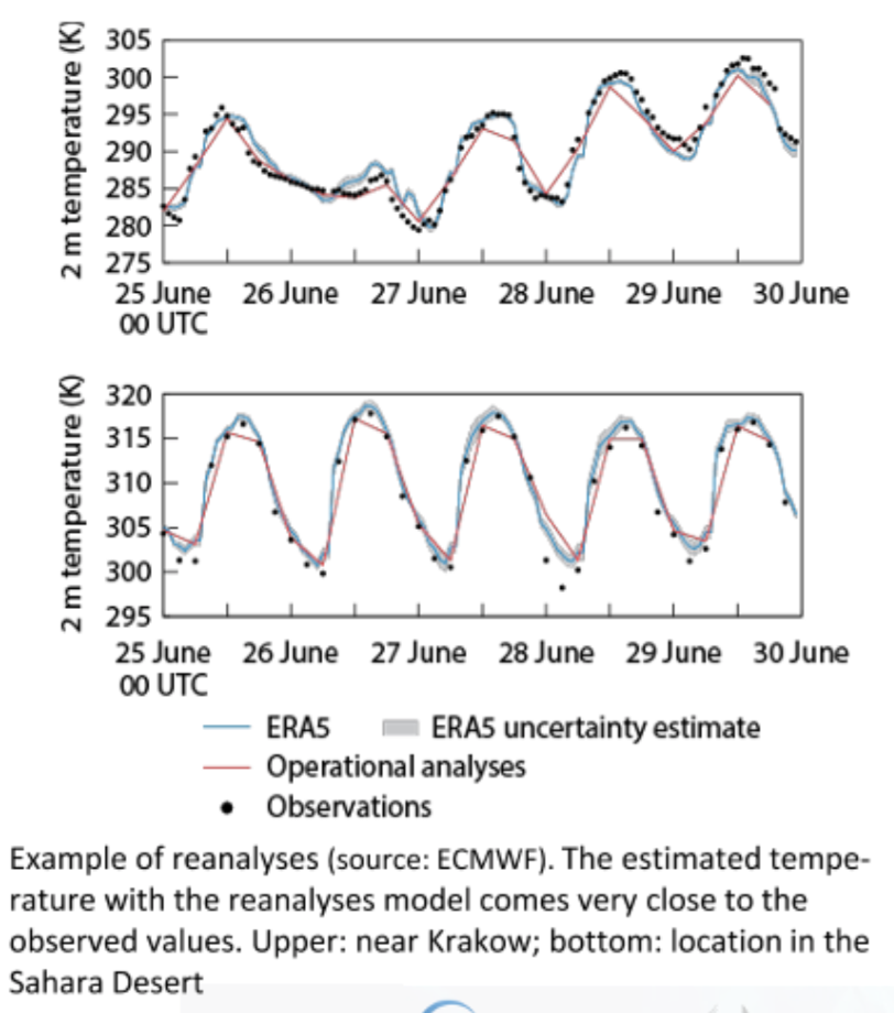
A climate reanalysis gives a numerical description of the recent climate, produced by combing models with observations (assimulation of observations in a climate model). It contains estimates of atmospheric parameters such as air temperature, pressure and wind at different altitidues, and surface parameters such as rainfall and soil moisture content. In the global re-analysis estimates are produced for all locations on earth, and they span a long time period that can extend back by decades or more.

Weather and climate (reanalysis) models vary in their use of data assimilation. Weather models assimilate observations only in the starting conditions of the forecast. Climate reanalysis models assimilate observations in the starting conditions as well, but also during the whole period simulated. This can only be done for the past climate where we do have observations.

For more information on re-analysis data and models that can be used in Europe, see the [dedicated chapter][regional reanalysis for Europe]

3.2.2.2 Seasonal to decadal predicitons (S2D)

Weather forecasts or predictions generally give information for up to two weeks ahead. Many sectors in society would like to know what the weather will be in one month, a year or a decade. E.g. will the coming season be dryer or warming than average? This is where S2D predictions come in. In S2D predictions, both initial values and boundary conditions are important.

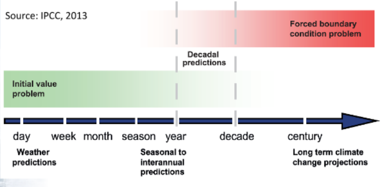
At lead times of weeks to months, predictions are typically initial value problems. “Climate” predictions such as seasonal outlooks, El Niño forecasts and seasonal hurricane outlooks fall into this category. The initial value is represented by the initial states of the climate system, including ocean heat content, and surface snow and ice cover. In this case, short-term evolution from an initial state is analysed with constant boundary conditions. Also, probability can be verified in time to provide meaningful feedback.

With projections, one looks typically at changing statistics in response to changing boundary values. In this case, the probability of projections cannot be given.

What will happen in the near future, up to a decade or two ahead, is the combination of natural variability and human-induced climate change. The next few years may be relatively cold, although the long term trend is increasing temperature. The next season may be extremely dry in a region, although the long term trend can be an increase in rainfall.

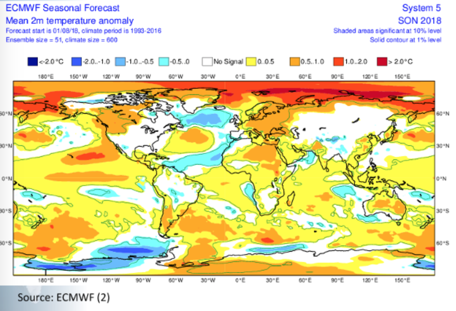
Example of a seasonal forecast: August 2018

The figure below shows how much colder or warmer the average temperature is expected to be for September-November 2018 compared to the period 1993-2016 based on several models. Whether one can rely on this forecast depends on the skill, which means whether we know that the forecast has added value of the longer term averages. For some regions this forecast has higher skill than for other regions. In the tropical regions there is a higher skill due to El Niño/La Niña.

3.2.2.3 Types of climate models

Climate models are often used to make projections for the future based on certain amounts of emissions (Representative Concentration Pathways, RCPs).

Among many different types of climate models, there are:

• Models that simulate the climate of the whole world (Global Climate / Circulation Model = GCM, Earth System Model = ESM)
• Models that simulate the climate only for a part of the world (Regional Climate Model = RCM)
• Models with more or less complexity/coupling. Some models only include the atmosphere (Atmospheric models), some models couple the ocean and atmosphere (coupled models). Earth System models couple even more systems.

There are more types of models which are used for specific climate research such as cloud studies on exchange of energy, humidity, etc. between the different air layers.

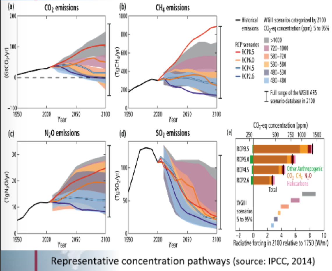
3.2.2.4 Emissions scenarios and RCPs

Emission scenarios are descriptions of how greenhouse gas emissions could evolve on various hypotheses. Emission scenarios are translated into GreenHouse Gas (GHG) concentration scenarios. These are used as direct input in climate models.

Currently 4 Representative Concentration Pathways (RCPs) are used. They are named after a possible range of radiative forcing values in the year 2100 relative to pre-industrial values (+2.6, +4.5, +6.0 and +8.5 W/m²). The RCPs are consistent with a wide range of possible changes in future anthropogenic (i.e. human) GHG emissions, and aim to represent their atmospheric concentrations:

• RCP2.6 corresponds to very ambitous climate policy, which probably leads to a temperature change of about 2 degrees Celcius compared to the pre-industrial era.
• RCP8.5 represents a scenario where few measures are taken and few technological breakthroughs are used.

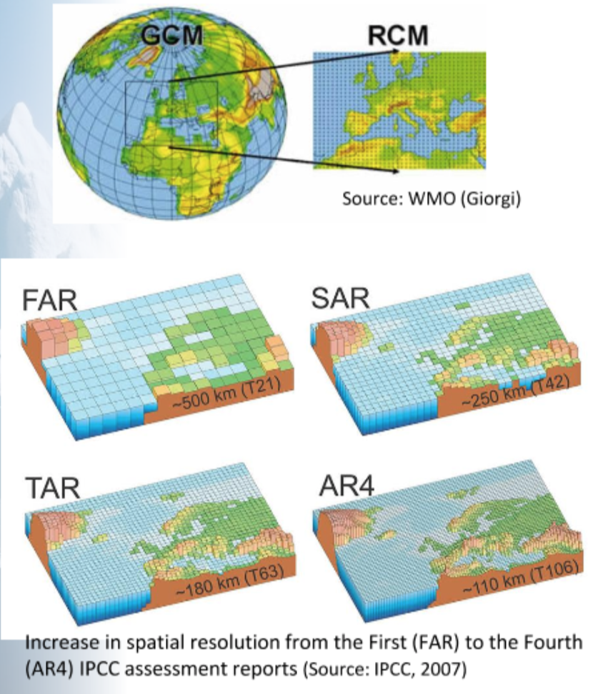
3.2.2.5 Global and Regional Climate Models

A Global Climate Model (GCM) is a numerical model representing physical processes in the atmopshere, ocean, cryosphere and land surface simulating the response of the global climate system to increasing GHG concentrations. GCMs depict the climate using a 3D grid over the globe. Different GCMs may simulate quite different responses to the same GHG emission scenarios, simply because of the way certain processes and feedbacks are modelled.

Regional Climate Models (RCMs) do a similar job as GCMs, but for a limited area of the Earth. Because they cover a smaller area, RCMs can generally be run more quickly (less computational power required) and at a higher spatial resolution than GCMs.

RCMs use information from GCMs at their boundaries (nested regional climate modelling technique). The driving data at the boundaries are derived from GCMs and can include GHG and aerosol forcing. ‘Regional’ in RCMs refers to regions as large as Europe or a large part of Europe. Currently many RCMs for Europe have a spatial resolution of about 25 x 25 km but also many simulations at 12 by 12 km are available. RCMs are used as a downscaling technique (from a coarser resolution of global models to higher resolution)

3.2.2.6 Climate Model Bias

Models are always a simplification of reality and therefore they will never represent reality exactly. In re-analyses we observed small differences between observations and model results. In climate models the differences may become clearly larger (also in S2D predictions biases will occur and will become larger with increasing time horizon).

Definition

Climate model bias are the differences in statistics of the observations for the reference period and the climate model simulation for the same period. It is determined by comparing the climate model output for a past period with observational data for that same period. This is illustrated in the figure below .

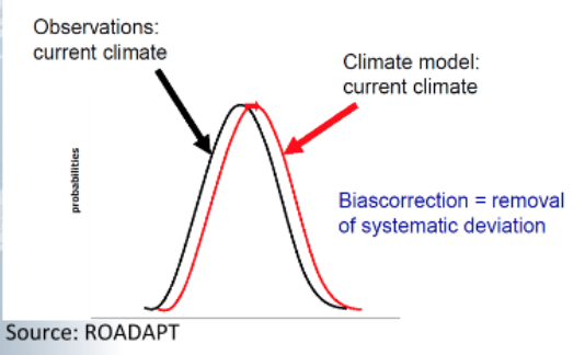
Figure of schematic representation of climate model bias: the systematic difference between model output and observations. The figure presents on the x-axis the daily temperatures in e.g. the month of July in the period 1981-2010 on a certain location. On the Y-axis the probability is shown. As can be see in the figure in the climate model, there is a systematic difference (higher temperature) between model output (red) and observations (black).

Model skill

Example applications: comparison of annual and seasonal climatological averages for relevant climate variables such as probability of extremes, variability, trends, etc.. The smaller the bias, the higher the model skill to simulate the observed climate correctly. The skill is often used as a measure of quality.

Biases are compared by comparing the statistics of observational records for a certain period (often 30 years) with the simulated climate for the same period in the past (for projections). Biases can not be determined by comparing e.g. the weather on certain dates or in certain years in the past.

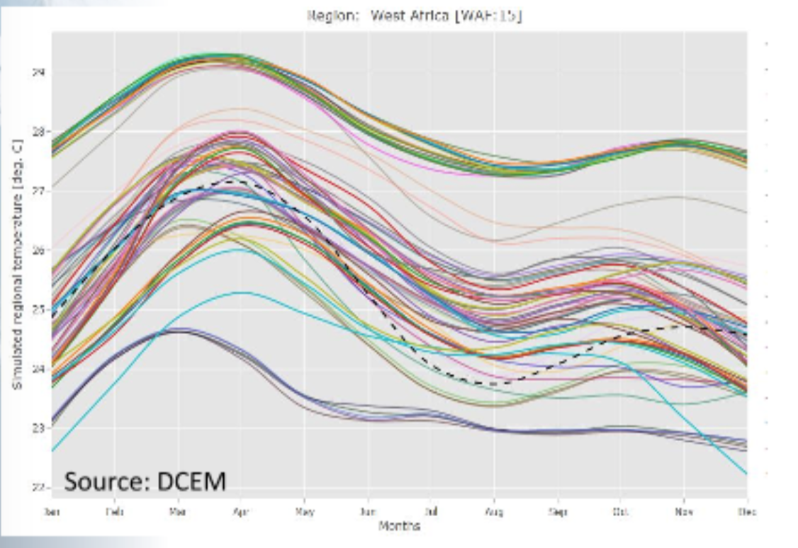
In the below figure, the annual cycle of the average temperature of West Africa for the period 1981-2010 from a large number of RCMs is compared with the annual cycle from the ERA-Interim re-analysis data (dotted black line; used as alternative for observations). Some models simulate the temperatures fairly well, whereas others have large biases.

Reasons for climate model bias

Some possible reasons are:

• Simplified physics and thermodynamic processes
• The way relations are described in numerical schemes (parametrization)
• Incomplete knowledge of climate system processes
• Limited spatial resolution in the climate model (horizontal and vertical)

Climate models produce area-average data, whereas many observations are point measurements. In order to determine the skill, climate model data should be compared with area-average data. This is especially important for climate variables where large spatial differences are observed within a grid cell, e.g. precipitation. For this reason, re-analysis data is often used to determine the skill of climate models.

The quality of climate data for the future cannot be assessed in a direct way, since no observational data set is available for the future. It is generally assumed that the bias/skill for the future is the same as for the past/current climate. When the skill is good for the current climate, we generally have more confidence in the results for the future.

3.2.2.7 Ensembles

Ensembles are a collection of model simulations characterizing a climate in the past, a prediction or a projection. Differences in initial conditions and model formulation or parameters result in somewhat different evolutions of the modelled system, and may give information on uncertainty associated with:

• type of model and initial conditions, in the case of climate forecasts

• type of model and scenario and internally generated climate variability, in the case of climate projections

Ensembles are usually made to characterize uncertainties (or variability). They need to be big enough to describe the relevant uncertainties or natural variability. The following uncertainties can be studied with the help of ensembles:

• Initial conditions: espacially important for forecasting and prediction. The initial conditions are slightly changed and the same model is run again (single-model initial condition ensemble). E.g. for the weather forecasting at ECMWF, 51 runs are made twice a day to determine the impact of the weather on the forecast. Having an initial condition ensemble can help to identify natural variability in the system. These ensembles are especially important for forecasting and predictions.

  

• Model descriptions of the physical processes (called ‘perturbed physics ensembles’): an ensemble of runs can be made with somewhat different parameter values in the same model, or even with different ways of describing various processes (including different resolutions, different climate models). Therefore, also a multi-model ensemble can be made.

• Forcings (emission scenarios): various RCPs are used as input for the climate projections. They represent the uncertainties about the future developments of socio-economic and technological developments (resulting in different emissions).

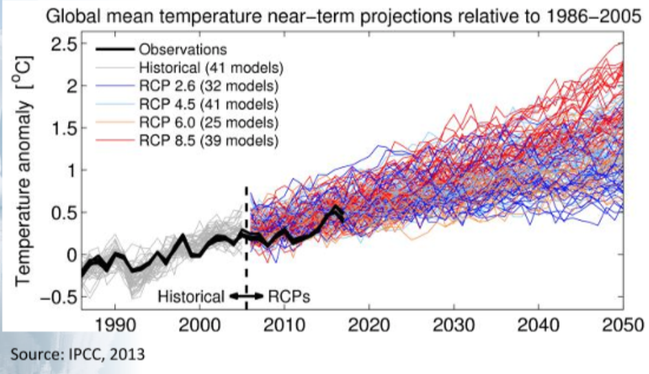
See below figure for an example of how ensembles are used to characterize and quantify various uncertainties. The grey lines present simulations with different climate models for the past. This helps to characterize the natural variability of the past and current climate. E.g. the red lines present the projections of different climate models for the highest RCP scenario. This helps characterizing the uncertainty about the climate (also called model uncertainty). The differences between the different colors (different RCPs) are used to characterize the uncertainty due to socio-economic and technological developments (also called scenario uncertainties).

3.3 Pro’s and con’s of different data sources

3.3.1 Advantages and disadvantages of different measurement types

	In situ stations (weather stations at land)	Data measurements at sea	Satellite data (radar and lidar)
Advantages	- Long time series. Some starting in 1850, from 1950 many more stations - Direct measurements of the ECVs	- Important for weather models, since they provide information for regions with a low density of observations - Direct measurement of ECVs	- High spatial coverage (also data for regions without ground stations) and high spatial resolution. - Data almost directly available
Disadvantages	- No equal distribution over the earth - Time series often contain ‘inhomogenieties’: apparent changes in climate due to e.g. the use of better instruments or changes in the environment.	- Ships and drifting buoys do not have a fixed location - No long time series at fixed locations	- No long time series yet (from about the end of the 90s) - The satellite signal has to be translated into the desired climate variable: this introduces additional uncertainties and ground observations are needed to make this translation. - Systematic disturbances in the signal due to the atmosphere

3.3.2 Advantages and disadvantages of different types of data

	Reanalysis data	S2D Data	Climate model data
Advantages	- Provide also estimates for climate variables where and when there were no observations - Provide area-average data, and therefore can be used to determine the skill of climate model projections/simulations and S2D predictions.	- Data for the near future (seasons to decade). - Because of the use of ensembles this data can also be used for characterizing the natural variability more accurately then with observations only.	- Provide data for past and future (and look much further into the future then S2D). - Because of the use of ensembles this data can also be used for characterizing the natural variability and to determine the probability of extremes more accurately than with observations only.
Disadvantages	- Many reanalysis data have a rather coarse spatial resolution - May also contain some biases, espacially where there are few observations that could be assimilated.	- Poor skill of S2D models in large part of Europe - Can contain biases, especially when forecasting for a longer period ahead.	- Presence of biases (various methods have been developed to correct for those) - Often relatively low spatial resolution (“downscaling” techniques have been used to get a higher spatial resolution)

3.4 References