Chapter 5 Climate Data Discovery
See also introductory video for this part.
5.1 Difference between weather and climate
For an overview of the basic differences between weather and climate (models), see the dedicated part in the first chapter. In short:
- Weather: conditions of the atmosphere over a short period of time
- Climate: average behavior of the atmosphere over relatively long periods of time (usually >30 years).
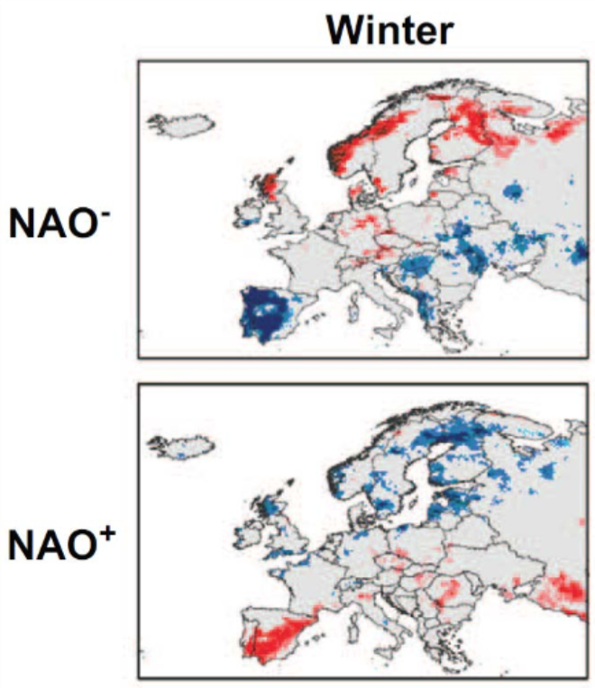
Climate variability is often expressed as anomaly, in months-seasons-years. Depending on the location, these can be influenced by e.g. the North Atlantic Oscillation (Europe) or El Niño/La Niña:
5.1.1 Weather and climate vs. decision making
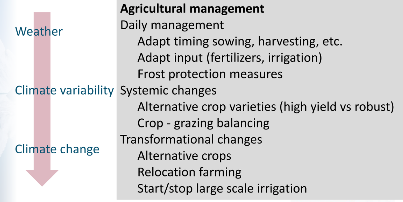
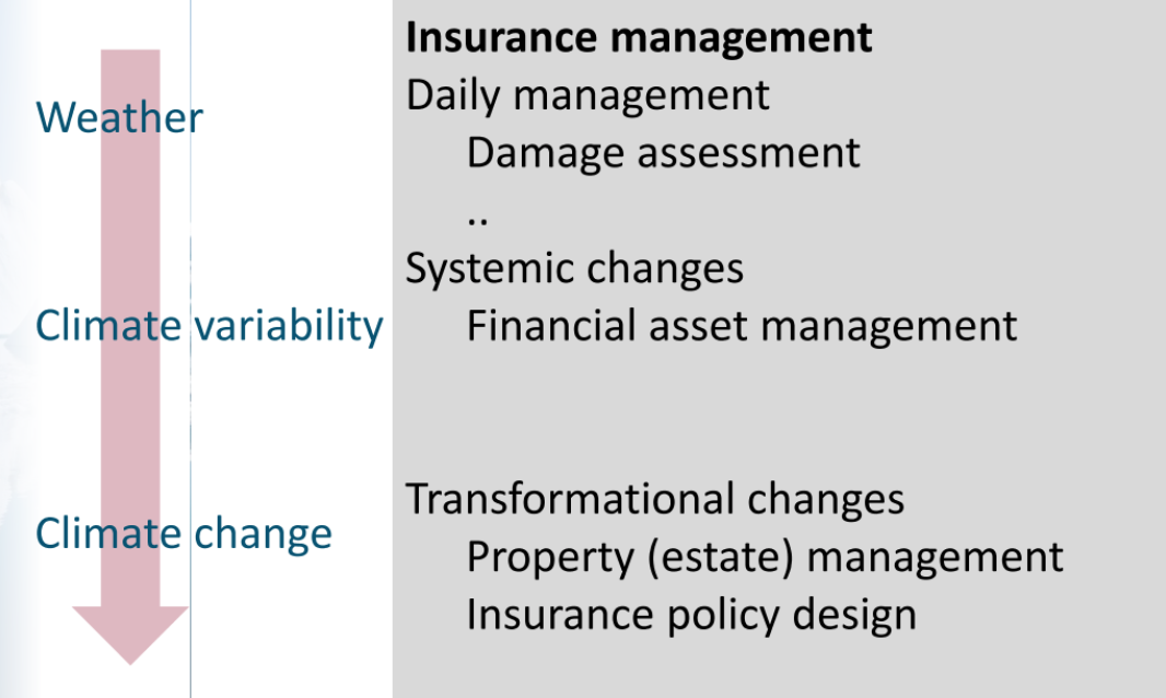
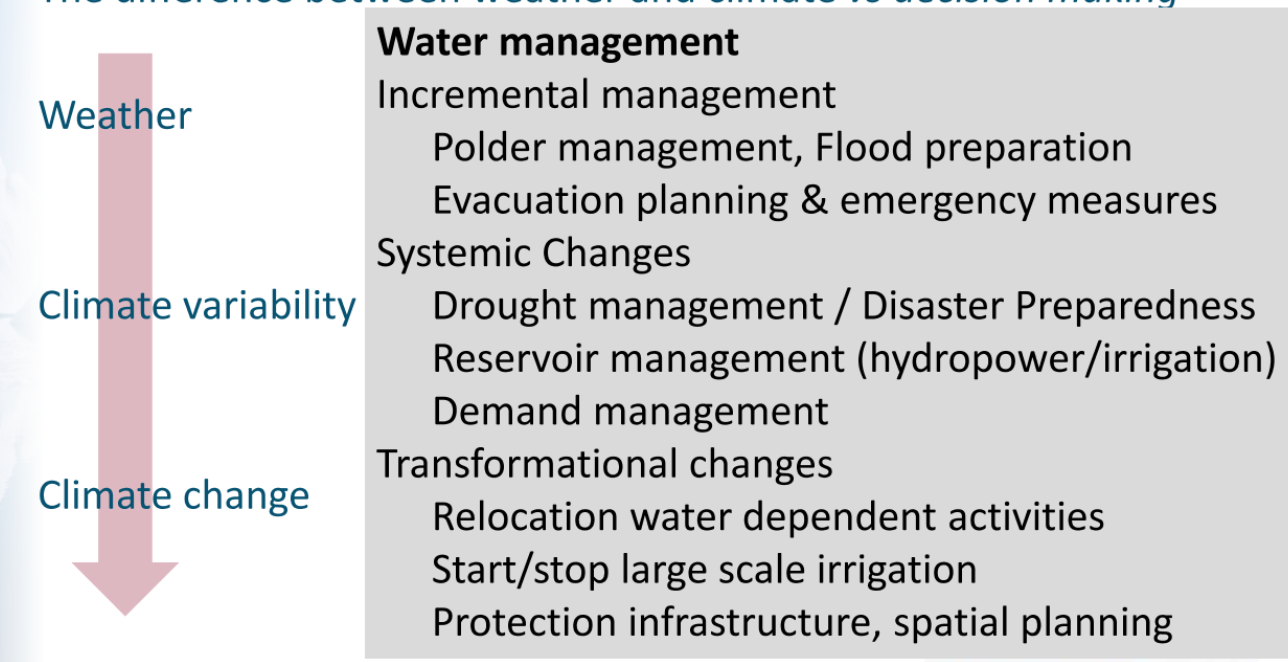
The types of data needed, depends on the topic/sector covered and type of decisions that need to be made. For example in the water sector, agricultural sector and insurance sector both weather (daily decisions), climate variability (systemic changes) and climate change (transformational changes) information could be needed:
info-ins
info-water
5.2 Different sources of climate data
See also the online video. This lesson goes further in depth on charateristics and utilisation cases of the different types of sources:
- In-situ (direct) observations (such as weather stations). For more information see the dedicated section in the first chapter.
- Satellite observations (indirect). For more information see the dedicated section in the first chapter.
- Reanalysis products. For more information see the dedicated section int the first chapter.
- Weather model forecasts
- Seasonal to decadal climate forecasts (S2D). For more information see the dedicated section in the first chapter.
- Climate change (model) projections. For more information see the dedicated section int the first chapter.
- Sectoral climate indices
5.2.1 Relations between the different data sources
Observations are needed for 2 things:
- Find the state of the atmosphere for a certain moment, from where to start model simulation development (= initial conditions)
- Observed data are needed for model development. Models are constantly validated and improved where needed.
5.2.2 Sources available on C3S
As in-situ measurements are rarely useful for climate (impact) assessments, the original data can only be found at the original provider. However, C3S provides gridded products of Essential Climate Variables (ECVs). For an overview of existing ECVs, see the dedicated part in the first chapter.
- Observations from global climate data archives
- Observations from baseline and reference networks
- Climate monitoring products for Europe
- Etc.
5.2.2.1 Observations
- In-situ observations
- Available at C3S from +- 1850
- Gridded observation products are available, e.g. Eobs, GPCC, …
- Satellite observations
- Available at C3S from +-1970
- Merged observation products available, e.g. GPCP
- Improved continuity, quality, …
- Other gridded products:
- Atmosphere (composition): Long-lived GHGs, ozone, aerosols, …
- Atmosphere (surface): precipitation, clouds, …
- Ocean (physics): sea surface temperature, …
- Land (hydrology): soil moisture, albedo, leaf area index, …
- …
5.2.2.2 Data produced by models: suited for particular time horizons
- Reanalysis products.
- available from 1950s
- remain close to the observation, advantage to be availble for all locations at any moment in time
- Continuous (hourly) data (space/time)
- good alternative to observations for regions with few observation points
- better than observations that are interpolated with geostatistical technique (discouraged!)
- Latest data available on C3S: ERAS (ERA5-Land, AgERA5), RRA, …
- Specialized high-resolution sets will become available as well.
- See separate lesson on reanalysis
- (Weather model forecasts)
- run from now —> 14 days future
- Seasonal [to decadal] climate forecasts (S2D)
- Seasonal: now —> +12 months
- Are ‘initialized’ climate models, NOT a weather forecasts
- Montly statistics have predictive skills, not hourly/daily time series
- Available at C3S (graphical + numerical): SEAS5/ECMWF, GloSea5/UKMO, System6/MeteoFrance, SPSv3/CMCC, GCFS1/DWD, CFSv2/NCEP, MRI-CPS2/JMA
- See lesson on seasonal forecasting products
- Decadal: now —> few decades
- Seasonal: now —> +12 months
- Climate (model) projections
- … —> +-1800 —> 2100 —> …
- Not initialized, NOT a weather forecast, and NOT a reanalysis —> they only have statistical meaning (to analyse difference between historic and future climate)
- Follow prescribed GHG emission scenarios (RCPs)
- Important to use multiple models and multiple RCPs
- Examples available at C3S: CMIP5, CORDEX, CMIP6 will be available soon.
These types of data can be used to derive specific sectoral impact indices. Sectoral impact models (water, agriculture, agriculture, energy, insurance, …) and data such as river discharge, crop development indicators, power potential, etc… are also available at C3S.
Bias correction may be needed, increasing from top to bottom of model data list (see lesson on bias correction).
5.3 Strategies to find the data you need: “Be specific”
See also the accompanying online video. The main message is: “Be specific” about:
5.3.1 Time horizon and region/location
- Most data are gridded, don’t follow political/sectoral classifications
- The time horizon depends on the problem to be adressed. It might be monthly or sub-daily.
- Choice can affect the base-period for change assessment (1961-1990, 1981-2010, …)
- Historical questions (can be very specific in place and time) versus questions about the future (generally larger areas & longer periods)
5.3.2 Source (observation or model-based)
- If from model: from which model, and which scenario?
- Often you need both: using observations/reanalysis to assess bias/skill of predictions/projections for chosen model, variable, location, season of interest, …
5.3.3 Variable of interest
- Each variable has different meaning and use
- Depends on the problem assessed:
- Time series (for impact model forcing) vs statistics. E.g. agriculture: “number of days with temperature below zero”, floods: “number of times a certain amount of rain falls in 500y period”. Statistics = climate impact indices. Time series can be used to feed your own model.
- Mean vs. extremes, percentiles vs treshold, single/combined —> generally agreggated from daily data
- Set of (standard) Climate Indices (CCI) = tools on CDS to compute those on demand.
5.3.4 Model selection
For more information about model selection, see the dedicated chapter below
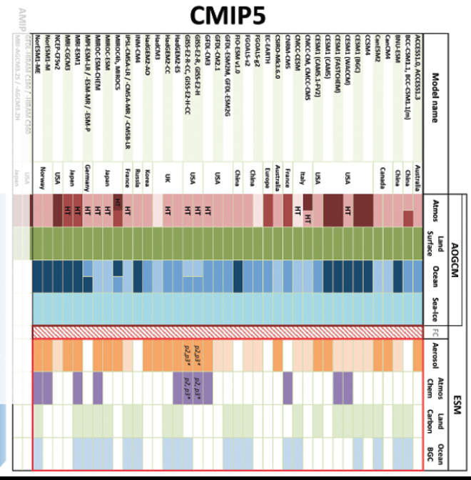
Which model to chose? In CMIP5: more than 40 models available. They differ in:
- Resolution
- Complexity and structure
- Parametrization
- Representation of earth system feedbacks (and strenths of those)
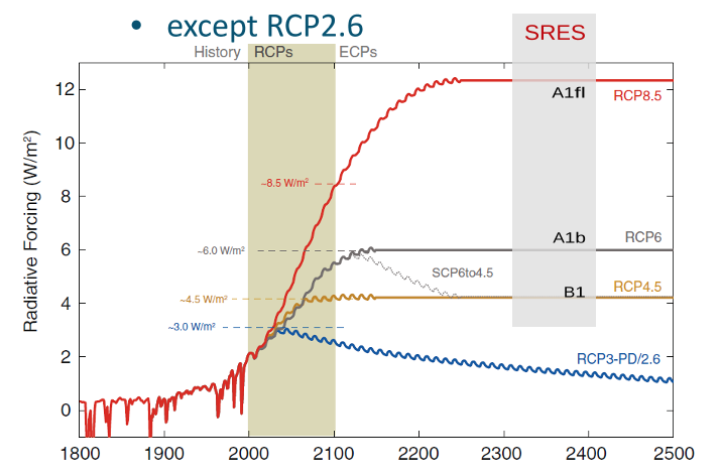
5.3.5 Scenario selection
Even though the UNFCCC in Paris agreed we should follow RCP2.6-scenario, you often need to assess more than one RCP or Shared Socio-Economic Pathway (SSP). Especially when you are interested in analysis for the end of the century.
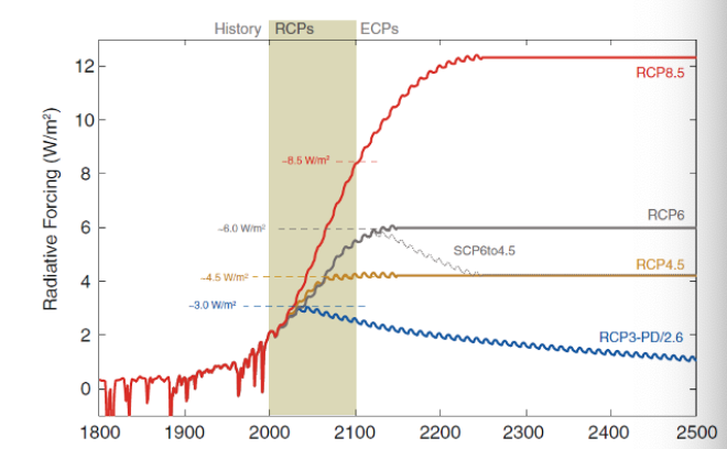
rcpexample
When you are only interested in changes in the next decades (<2050), choices in RCP-SSP become less relevant.
5.3.6 Model selection for seasonal forecast
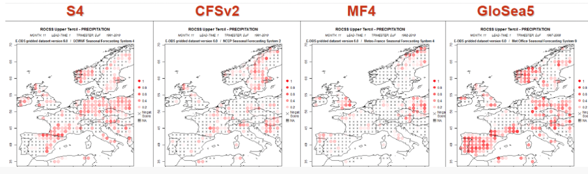
Since the predictive skill of models are complementary (region, lead time, …), it is recommended to use a combined product: the Multi-Model Ensemble.
See also lesson on uncertainty below.
5.3.7 References
- Eumetsat infrared image 31 July 2018 1500hrs. Link
- Köppen climate classification of Europe. Link.
- Nobre, G. G., et al. (2017). “The role of climate variability in extreme floods in Europe.” Environmental Research Letters 12(8): 084012, DOI: 10.1088/1748-9326/aa7c22
- ECMWF
- GPCC Vizualizer. Link.
- C3S_312a_Lot3_TVUK_2016SC1 - Product User Guide and Specification, p8
- C3S_312a_Lot6_IUP-UB – Greenhouse Gases - Product User Guide and Specification (PUGS) – Main document , p32
- IPCC-AR5 WG1, Table 9.1 Flato, G., et al. (2013): Evaluation of Climate Models. In: Climate Change 2013: The Physical Science Basis. Contribution of Working Group I to the Fifth Assessment Report of the Intergovernmental Panel on Climate Change [Stocker, T.F. et al. (eds.)]. Cambridge University Press, Cambridge, United Kingdom and New York, NY, USA.
- RCP figure: Meinshausen, M., et al. (2011). “The RCP Greenhouse Gas Concentrations and their Extension from 1765 to 2300.” , DOI: 10.1007/s10584-011-0156-z
- SSP Figure. Link.
5.4 Strategies to find the data you need: Climate data processing chain (Advanced)
See lesson Climate Data Discovery - Advanced Level : link
5.4.1 Overview of climate processing chain
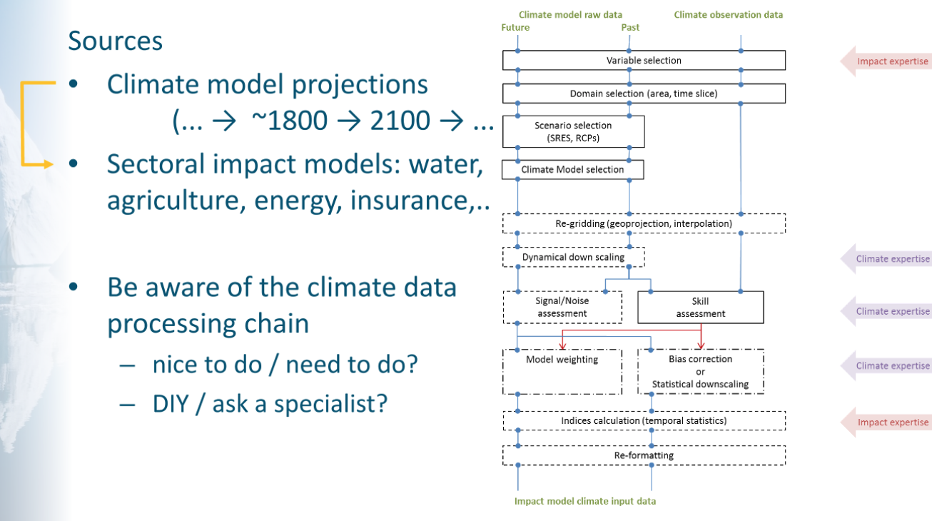
chain-overview
Note: sectoral impact studies mostly bypass the part between domain selection and re-formatting, but nevertheless important to know the details.
5.4.2 Variable Selection
- Near surface data (single level)
- Higher atmosphere (pressure levels)
- Near surface is NOT level 1000hPa:
- Strong gradients with height in boundary layer
- E.g. Tair_2m, Wind_10m
- Beware of (extreme) extremes
5.4.3 Domain selection
- Not too small
- sampling variance
- sampling gradienst
- Relatively simple BC/DS-method is sufficient
- Beware of sharp gradients
- Coast line vs. model land mask
- Steep topography
- Large land use contrasts
5.4.4 RCPs and SSPs
Main message: be consistent.
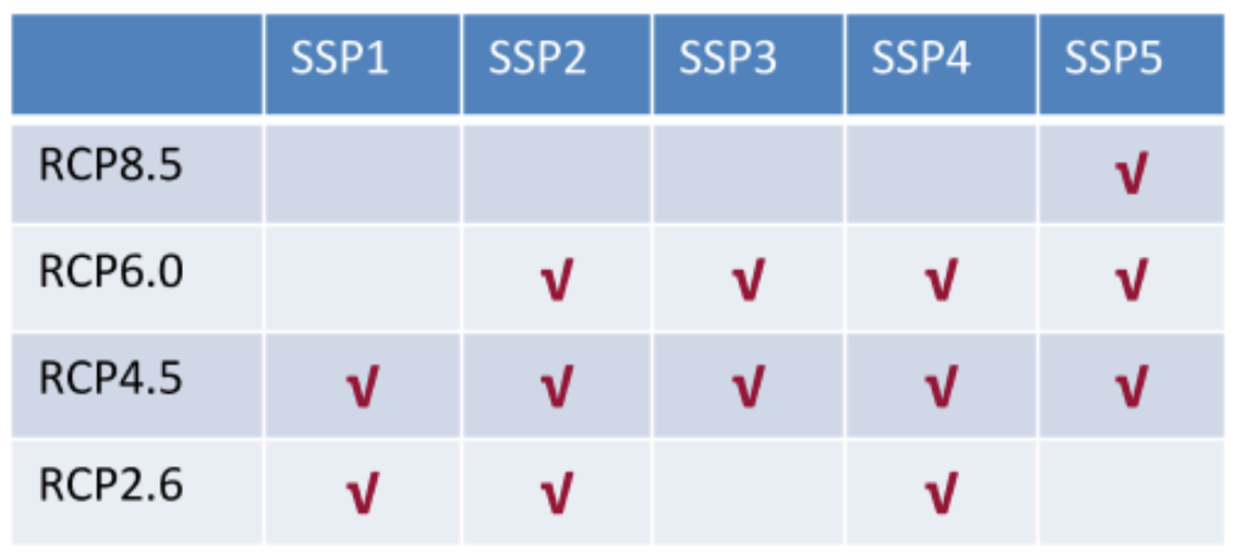
rcp-ssp-consistency
4 RCPs set by IPCC-AR5 (depending on radiative forcing, depending on GHG concentrations). IPCC-AR4 similar, before: SRES (except RCP2.6)
4-rcps
5 Shared Socio-Economic Pathways (SSPs). Similar in IPCC-AR4, before: SRES
5-ssps
5.4.5 Climate model selection: how to distinguish? (climate sensitivity, transient response, (dis)similarity, spatial scale, …)
For more information about model selection, see the dedicated chapter below
40+ GCMs: different resolution, complexity, parameterisations, feedback strenghts, etc..
Consider (equilibrium climate sensitivity) ECS/ (transient climate response) TCR
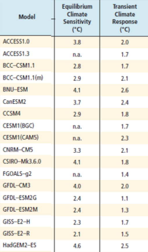
ecs-tcr
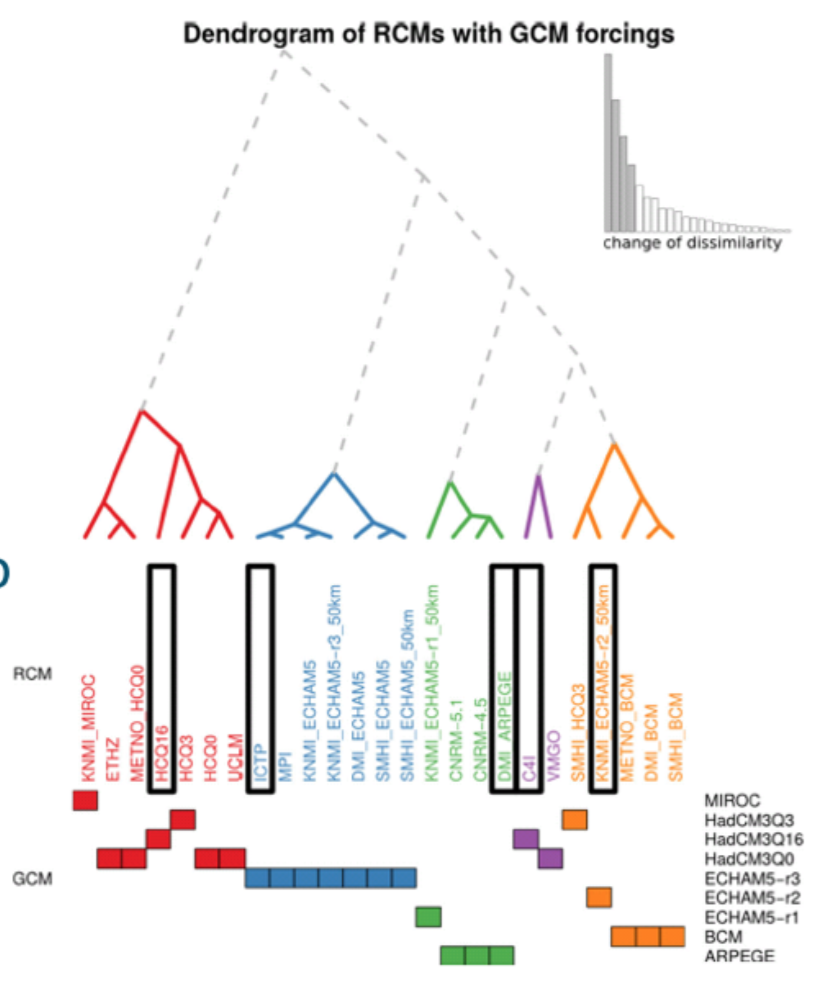
Consider model (dis)similarity:
model lineage and model behaviour
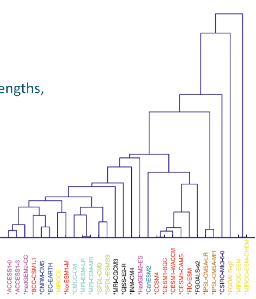
model-lineage
local spread in #T-#P
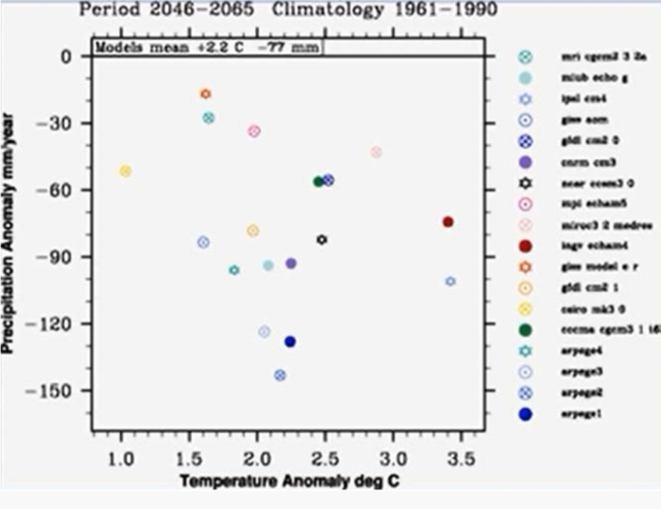
local-spread
Consider area:
for small areas pick model with best skill
model-skill
At larger spatial scales: Multi-Model Ensembles (MME) show better than single model
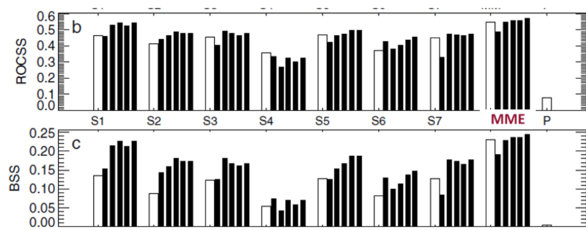
multi-model-skill
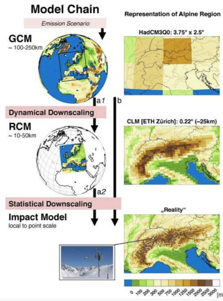
5.4.6 Dynamical and statistical downscaling
For more information about bias correction and the importance, see the dedicated chapter further on
5.4.6.1 Why downscaling?
GCM/ESM low resolution:
- Poor spatial gradients (topography, coast lines, land use, megacities)
- Poor extremes (esp. precipitation)
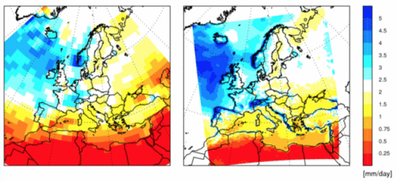
downscaling1
5.4.6.2 How to do downscaling?
- RCM higher resolution, limited area
- Needs nesting in GCM/ESM
- (statistical downscaling)
downscaling2
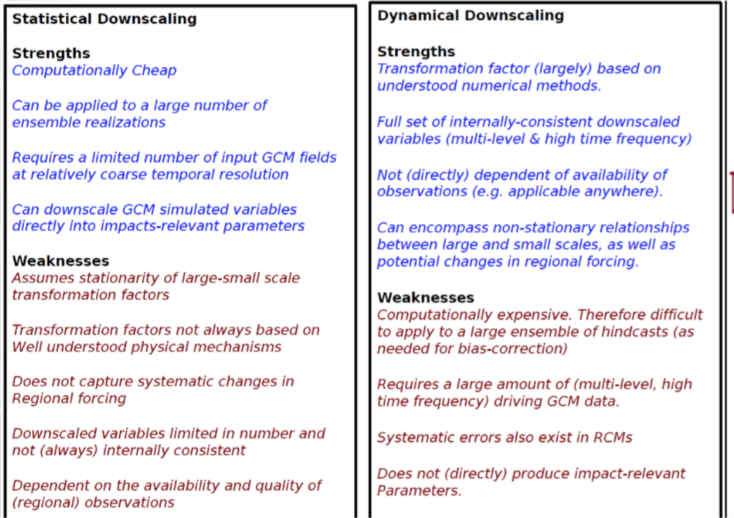
5.4.6.3 Statistical and Dynamical downscaling
Dynamical downscaling: uses high-resolution climate models for a regional sub-domain, often using lower-resolution global climate models as boundary conditions
Statistical downscaling is a 2-step process:
- Statistical relationship is derived between observed small-scale variables and larger global climate model scale variables
- Statistical relations are used to estimate the future climate at the smaller scale based on the largescale variables from GCM projections of the future climate.
statistical-dynamical
Dynamical downscaling: regional climate model uses the global clmiate model (GCM) as boundary condition:
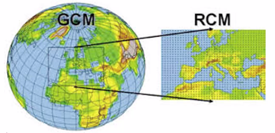
rgm-to-gcm
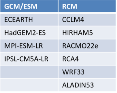
GCM / RCM selection
IPCC-AR5 / CMIP5: 40+ GCMs
IPCC-AR5 / CORDEX: many RCMs
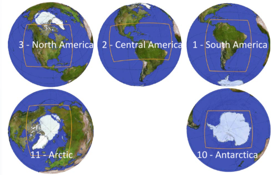
- Each region (generally) sparse matrix 2-5 GCMs x 2-5 RCMs (e.eg. Europe 4x6 = +- 18)
- delta-x = +- 44 km / 11 km
For selection:
Consider ECS/TCS (similar to parent GCM)
Consider model (dis)similarities
dissimilarities
dyanmical-downscaling
gcm-rcm-combined
Statistical downscaling: statistical model is used to transform a GCM result to a result at local scale:
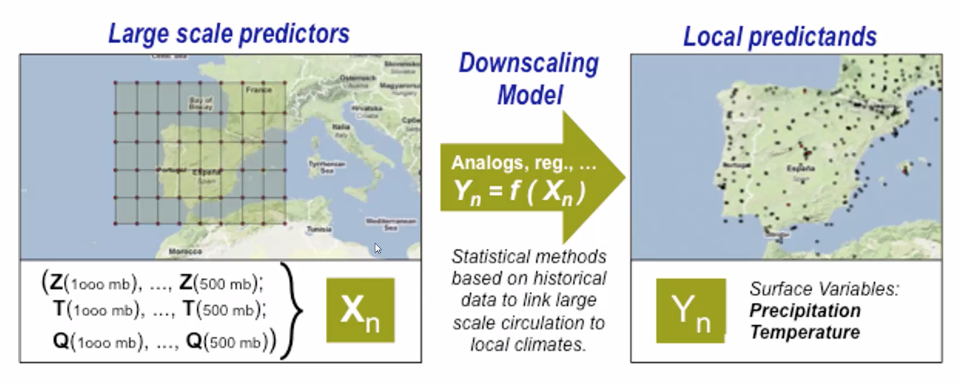
statistical-downscaling-theory
5.4.7 Skill assessment, model weighting and bias correction
- All ESM/GCM/RCM have systematic biases: vary by model, region, season, parameter…
- Can be corrected to some extent
- Small biases give ‘trust’:
- Model selection (yes/no)
- Model weighting (continuous)
- Statistical downscaling and bias correction = technically very similar (see lesson on bias correction)
5.4.8 Indices calculation (temporal statistics) for different variables
- Be specific: varirable of interest
- Depends on the problem assessed:
- Time series for impact model forcing vs. statistics
- Mean vs. extremes, percentiles vs tresholds, single/combined, … (generally aggregated from daily data)
- Set of standard climate indices (CCI)
- Temperature: TG, TX, TN, …
- Cold extremes: TG10p, FD, CFD, …
- Warm extremes: TG90p, SU, CSU, WSDI, …
- Precipitation: RR, RR1, …
- Dry extremes: SPI3, SPI5, CDD, …
- Wet extremes: R95p, R99p, R20mm, RX1d, RX5d, CWD, …
- Others:
- Wind: FG, FXx, FG6Bft, DDeast, …
- Biological: BEDD, GSL, HI, …
- Combined: WW, WD, CW, CD, TCI, …
- Pressure: (PP, NAO, ..), SST (ENSO, PDO, …)