Chapter 4 Climate data from models
Introductory video by Rob Groenland from KNMI Netherlands.
For more information about model selection, see the dedicated chapter below
4.1 What is a climate model?
- For a basic explanation of climate models, see the section on climate models in lesson 1.
- For an explanation of the difference between weather and climate (models), see the dedicated section in lesson 1.
- For a basic overview of types of climate models, see the dedicated section in lesson 1.
- For a basic overview of definitions and differences between global and regional climate models, see the dedicated section in lesson 1.
4.1.1 Complexity of climate models
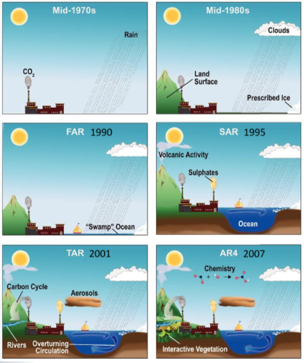
For decades scientists have been using mathematical models to help us learn more about the Earth’s climate. Over time these models have increased in complexity, as separate components ahve been merged to form coupled systems. The figures below shows the evolution of such systems (first figure from NASA, second figure from IPCC, 2007)
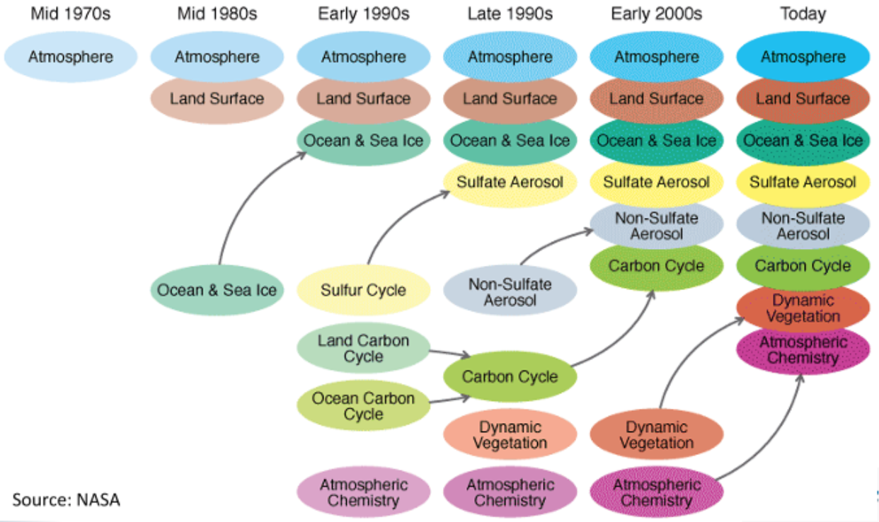
4.1.2 Earth System Models
Earth System Models (ESMs) represent advanced and complex descriptions of the Earth’s atmosphere, ocean, land and surface. The figure shows the difference between a climate model and an ESM. The componenets in green boxes (biochemical) makes a climate model an ESM.
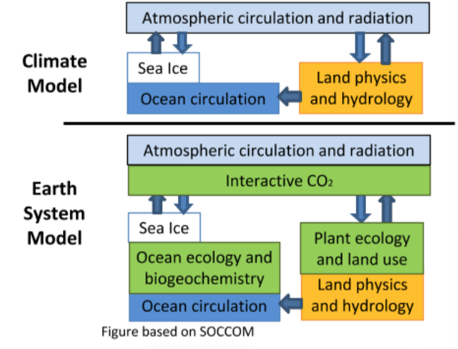
Major advances to climate models and ESMs skills have been made through improving parametrization of processes (parametrization: method of replacing processes that are too small-scale or complex to be physically represented in the model by a simplified process). By modelling new feedback processes, the number of processes and complexity in the models has increased. For example: the addition of carbon storage in the ocean and land surface, affecting the carbon cycle response to GHG induced climate change.
4.1.3 Spatial and Temporal Resolution
Although we know that climate variables such as temperature vary continuously over the surface of the Earth at each moment, calculating such properties for the entire globe and for each moment is beyond the reach of even the fastest supercomputers.
- Spatial resolution: specifies how large (in degrees of latitude/longitude or in km/miles) the grid cells in a model are. Not every horizontal layer has the same thickness: close to the earth’s surface more detail is required. A typical global climate model might have grid cells with a size of about 50-100 km, although now researcherse are also starting to make simulations with grid sizes of 25 km.
- Temporal resolution: refers to the size of the time steps used in the models and how often (in simulated or “model time”) calculations of the various properties are being modelled. Although the data are often not saved for future use, often time steps of 1 hour are used.
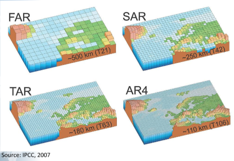
4.1.3.1 Increase of spatial resolution
The figure below shows the increasing spatial resolution of climate models used through the first four IPCC assessment reports: first (“FAR”) published in 1990, second (“SAR”) in 1995, third (“TAR”) in 2001 and fourth (“AR4”) in 2007. In the fifth report from 2014 the resolution of several global models was about 50 km (IPCC, 2013). The increased spatial result was a result of increased computing power and a request for better representation of all kind of climate effects, including extreme events.
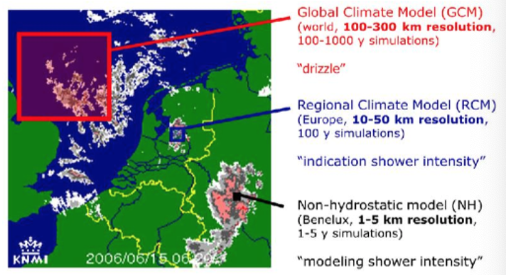
4.1.3.2 Example of impact of high spatial resolution
In this figure the sizes of the grid boxes in a GCM and RCM are shown. Climate models produce area average information. Therefore, the rainfall in the GCM grid box is on average over the whole grid box not more than drizzle. The chance that there will be rainfall in the whole are of a RCM grid box at the same moment is much higher. Therefore, RCMs will give a better indication of shower intensity (and spatial differences).
Non-hydrostatic weather forecast models use a much higher spatial resolution and, therefore, give a better indication of shower intensity.
4.2 Differences between climate projections, predictions and scenarios
Climate
A climate projection is the response of the climate system to different GHG scenarios, often based upon simulations with climate models. The emissions/concenttration/radiative forcing scenario used is based on assumptions, that may or may not be realized, and are therefore subject to substantial uncertainty not related to the climate system.
A climate prediction or climate forecast is the result of an attempt to produce a most likely description or estimate of the actual evolution of the climate in the future, e.g. at seasonal, interannual or decadal time scales. While seasonal forecasts are routinely issued in some regions, climate predictions at longer time-scales are still at an early research stage, for example within the CMIP5 climate modelling community. In the same way as weather forecasts depend on the initial state of the atmosphere, climate predictions depend on an accurate description of the initial state, mainly in the oceans. In contrast to climate projections, climate prediction rests on initial simulations of observerd conditions and is limited to time scales from subseasonal to decadal. Subseasonal to decadal predicitons (S2D) - explained in the related section in chapter 1 - is also known as climate prediction.
As mentioned in the related section in chapter 1 on subseasonal to decadal prediction, predictions are typically initial value problems. In this case, short-term evolution from an initial state is analysed with constant boundary conditions. Also, probability can be verified in time to provide meaningful feedback. While with projections, one looks typically at changing statistics in response to changing boundary values. In this case, the probability of projections cannot be given.
Weather
A weather forecast predicts the state of the atmosphere over a short period of time - for Europe usually up to about two weeks - and is independent of the initial state of the atmosphere (and the upper ocean). The initial state is obtained by means of the global network of meteorological stations and observing systems.
4.2.1 Climate scenarios
A climate (change) scenario is an image of a potential future that is based on knowledge of the past and assumptions on future change. The IPCC scenarios are based on a clear logic and a data-driven storyline (or narrative) of what events have occured in the past and how the future may unfold. A climate change scenario is the difference between a climate prediction and a reference period in the past (e.g. 1981-2010). The term “climate scenario” is also regularly used for individual climate projections.
Climate (change) scenarios are generally based on climate projections that use GHG emission or concentration scenarios:
4.2.2 Emission scenarios and RCPs
For an overview of emission scenarios and RCPs, see the dedicated section in the previous chapter.
4.3 How is the quality of models evaluated? (what is a climate model bias?)
4.3.1 Climate model bias and model skill
For a definition of climate model bias, the link between model bias and model skill and an overview of reasons for climate model bias, see the dedicated part in the previous chapter.
4.3.2 Types of climate ensembles
For an overview of (the different types of) climate ensembles and examples of those, see the dedicated section in the previous chapter.
4.3.3 Climate Model Intercomparison Project (CMIP)
There are many institutions involved in developing and running their own climate models. Although they all base their models largely on the same existing knowledge of the climate system, there are also differences in e.g. how certain processes are described, which data are used for calibration of the models, etc.
In 1995 the Coupled Model Intercomparison Project (CMIP) started. CMIP is a framework for coordinated climate model experiments, allowing scientists to analyse, validate and improve GCMs in a systemic way. “Coupled” refers to the fact that all included models are coupled atmosphere-ocean GCMs. This video from the World Climate Research Programme gives an overview of the CMIP.
Data from the fifth CMIP project were used extensively in the IPCCs 5th Assessment Report (IPCC, 2013, 2014) for:
- Improving the understanding of climate and assessing the mechanisms responsible for model differences
- Making projections for the future for policy makers and adaptation research
- Evaluating how realistic the different models are in simulating the recent past
4.4 The use of climate model data
Climate model data have clear advantages over observations. The most important are:
- Data can be provided for locations and periods without observations
- Climate models are the only source that can be used for the future
- Climate model ensembles can provide more information for the past/current climate and for the future with which uncertainties and natural variability can be estimated.
To use them in a correct way, one should be aware of the limitations and assumptions behind the data too.
4.4.1 What climate model data are available?
Climate data for the past/current climate:
- Climate model simulation (projection) runs. When making a run for the future, always a run for the recent past is made.
- Reanalysis (see dedicated part in previous chapter)
Climate data for the future:
- Climate model simulation (projection) runs, for various emission/concentration scenarios (RCPs)
- Seasonal to Decadal Precitions (S2D) (see dedicated part in previous chapter)
In most cases observational data are also needed to use the climate model data (e.g. to determine the skill/bias).
Reanalysis data are often used as alternatives for observations. Reanalysis provide a coherent and consistent description of the status of the atmosphere and ocean at all locations and dates. Moreover, they can provide area-average data that can be compared more directly with climate model projections.
4.4.2 Names of climate model data files
Names of climate model output files may seem very complicated. However, they are always build up in a systematic way containing at least the following information:
- Institute that made and runs the model
- Model name
- Period simulated
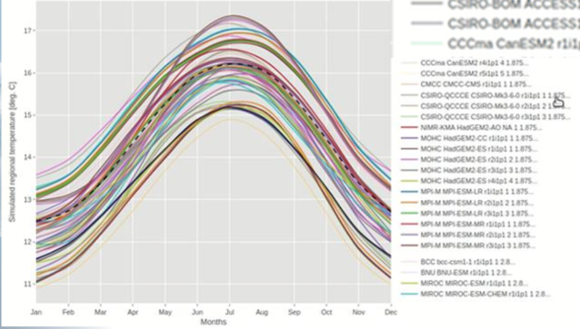
For example, in the figure below the first part of the first name refers to the institute (CSIRO-BOM: Australian institute) and the second part refers to the model used (ACCES). The figure shows an example of the average historical global temperature (1981-2010) over a eyear as simulated by many GCMs. In the C3S Climate Data Store (CDS), the model name is given with the institute and country in brackets.
4.4.3 Names of climate variables
Specific codes are used for climate variables. To be able to extract correct data from climate model data you have to know the codes or check them. This is also true for derived climate indices. Some examples:
| Code | |
|---|---|
| TN or Tasmin | minimum daily temperature |
| P or RR | daily or hourly precipitation |
| FF | wind speed |
| TXx | maximum value of daily maximum temperature (°C) in a season, month or year |
| RX1day | highest 1-day precipitation amount (mm) in a season, month or year |
Always check the dimensions of climate variables e.g. m.s-1 or km.h-1 for wind speed.
See for example for the names of derived variables the data dictionary of the European Climate Assessment Dataset (ECAD).
4.4.4 Assumption on bias
Before selecting or using climate model data, one should check the skill of the model. For this purpose, the climate model run for the past is compared with the observations (or reanalysis).
Below figure is an example with many different climate models for the average temperature for the period 1981 - 2010 - for South Europe/Mediterranean. The dashed line is based on reanalyses.
In climate research it is generally assumed that the bias will remain the same in the future, although this cannot be checked. Biases may not be the same throughout the year and they may not be the same for averages and extremes. There are different methods to remove the biases (not treated here). Bias correction datasets are also available for some climate model runs in the EURO-CORDEX project.
4.4.5 Use one or more projections?
The user of climate projections or climate scnearios should not trust the results of only one climate projection or scenario for impact analyses, as there is no such thing as ‘best GCM’, ‘best RCM’ or ‘best climate scenario’. Therefore, it is advisable to make use of a group of projections (ensemble) or a set of climate scenarios. Depending on which uncertainties one wants to take into account, a different ensemble should be selected. Only in cases where one wants to check whether climate changes are relevant at all, it could be sufficient to just use one projection or scenario (e.g. with the highest change in the relevant climate variable).
When using an ensemble or a selection of scenarios or climate model runs, take care that the relevant uncertainties are spanned. The climate data evaluation tool (DCEM; under development) developed by C3S is very useful to see which model runs have a high or low change in the future.
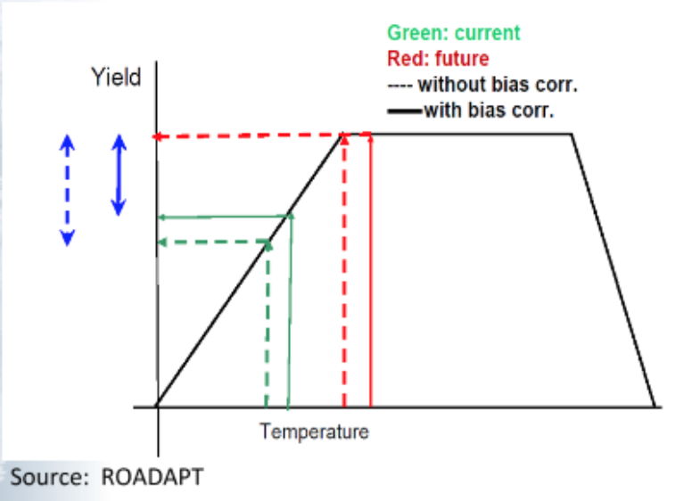
4.4.6 Importance of bias correction
Since climate model runs always contain biases, you cannot get an idea of the changes in the future by comparing observations directly with the uncorrected climate model projections for the future. To get an idea of the changes in the future you have to compare the climate model run from the recent past with the climate run of the future. In case of impacts you often have to bias correct the climate model runs first.
Below is a schematic example of the possible effect of climate model bias on the estimation of the impact of climate change. The climate model output has a systematiclly too low temperature. Since the impact model has a treshold and a non-linear relation with temperature, one makes an overestimation of the impact of climate change on yield without bias-correction.
4.4.7 Spatial resolution and downscaling
Downscaling is a general concept that embraces various methods for increasing the spatial resolution. Basically, there are two fundamentally different approaches to this:
- Dynamical downscaling: makes use of a Regional Climate Model (RCM) having higher spatial resolution
- Statistical or empirical downscaling: uses observations at local and coarser scales to determine the relations between them. These relations are then used to translate the information on coarser scales which are available only in e.g. GCMs to get information at higher spatial resolutions.
4.4.8 Required spatial resolution
Depending on the purpose of the use of climate data and the area that should be covered, one can use GCM or RCM.
For example, when looking at water management in the Iberian Peninsula, one wants to have relative high spatial detail. RCMs do have a higher spatial resolution and are therefore probably the most logical choice. When looking at world food security, data for the whole globe are needed and therefore GCMs will probably be used.
4.5 Developments in climate model research
Climate models are constantly being improved. When using climate data, always check the newest available data sets. Some subjects of current climate research are:
- More complex models (more components, ESM)
- Resolution increases in GCMs (e.g. Primavera project) and RCMs (e.g. EURO-CORDEX)
- How to improve the simulation of past trends? When models can simulate trends well, we can have more trust in simulated projections.
- How to make evaluation of climate models easier (development of tools) and how to evaluate more aspects of climate such as natural variability and extremes.
4.6 References and Links