Chapter 12 The ANOVA Approach to the Analysis of Linear Mixed-Effects Models

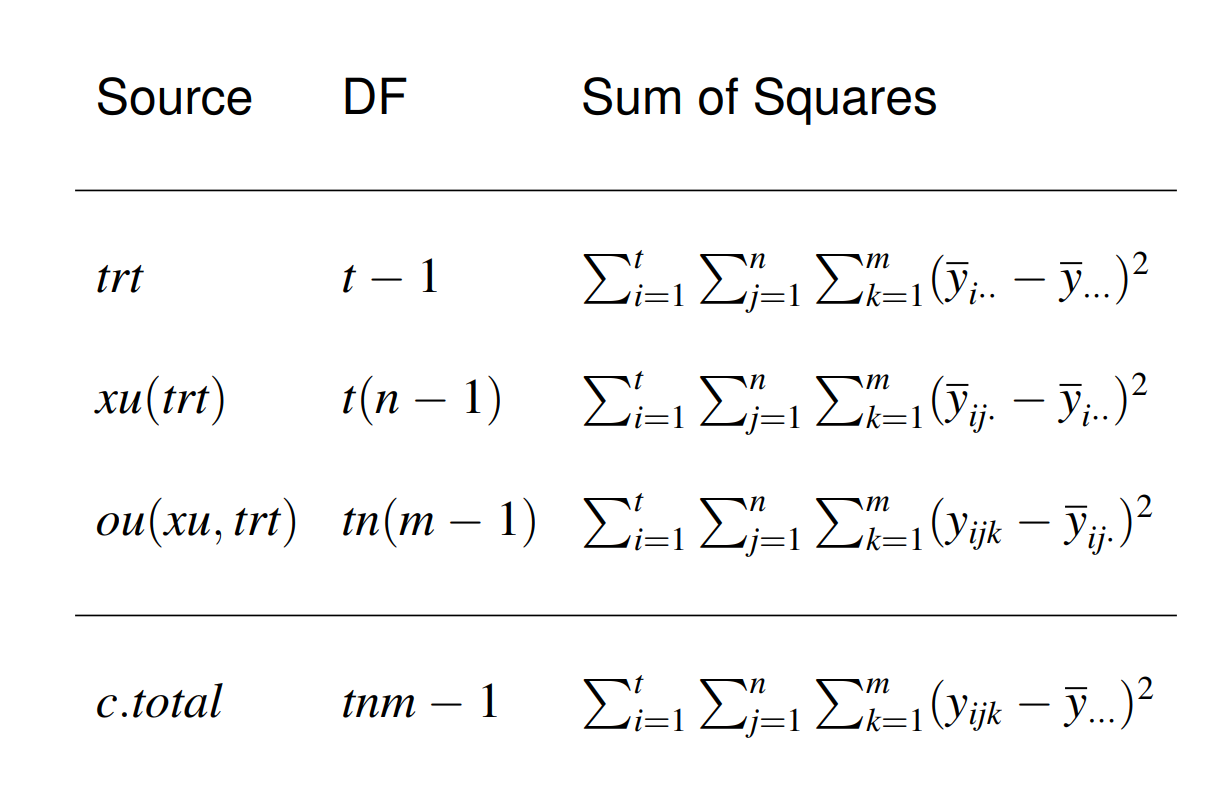
Suppose $y_{ij} = \mu + \tau_i + u_{ij} + e_{ijk}$ , $i = 1, \ldots, t; j = 1, \ldots, n; k = 1, \ldots, m$ . $\beta = (\mu, \tau_1, \ldots, \tau_t)'$, $u = (u_{11}, u_{12}, \ldots, u_{tn})'$, $e = (e_{111}, e_{112}, \ldots, e_{tnm})'$.

$$\begin{bmatrix}u \\ e \end{bmatrix} \sim N(\mathbf{0}, \begin{bmatrix} \sigma_u^2I & \mathbf{0} \\ \mathbf{0} & \sigma_e^2I \end{bmatrix})$$

• This is the standard model for a CRD with $t$ treatments, $n$ experimental units per treatment and $m$ observations per experimental unit.
• We can write this model as $\mathbf{y} = \mathbf{X\beta} + \mathbf{Zu} + \mathbf{e}$ where $X = [\mathbf{1}*{tnm\times 1}, I*{t\times t} \otimes 1_{nm \times 1}]$ and $Z =[I_{tn\times tn} \otimes 1_{m\times 1}]$.
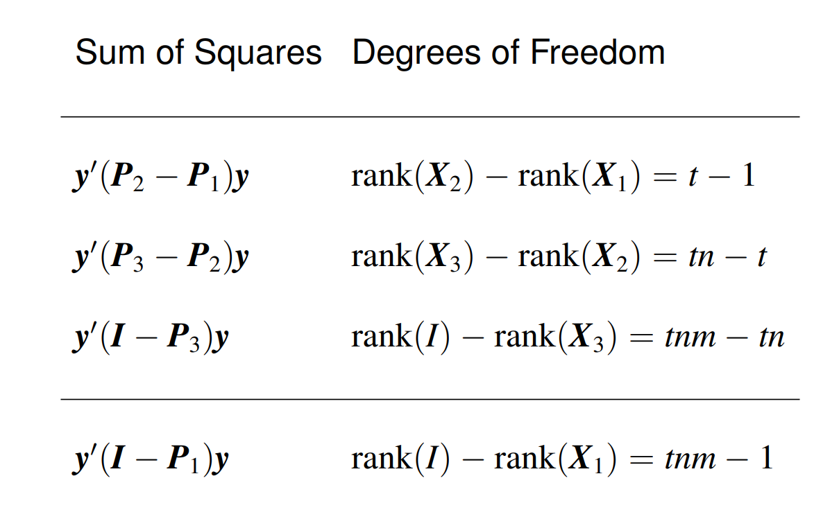
• Let $X_1 = \mathbf{1}*{tnm\times 1}$, $X_2 = X$ and $X_3 = Z$. Note that $\mathcal{C}(X_1) \subset \mathcal{C}(X_2) \subset \mathcal{C}(X_3)$. Let $P_j = P*{X_j}$ for $j = 1, 2, 3$.

• Suppose $w_1, \ldots, w_k \stackrel{ind}{\sim} (\mu_w, \sigma_w^2)$, then $E\{\sum_{i = 1}^k (w_i - \bar w_.)^2\} = (k-1)\sigma_w^2.$

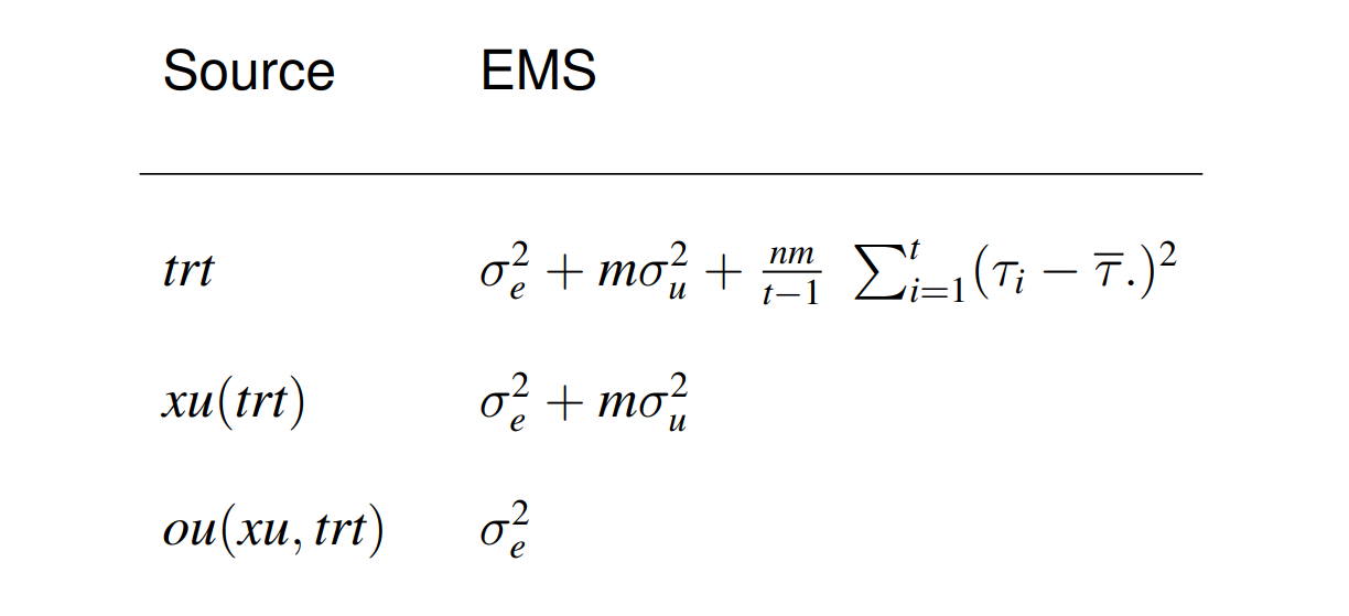
• Expected value of $MS_{trt}$:

  $$\begin{aligned}E\left(M S_{t r t}\right) &=\frac{n m}{t-1} \sum_{i=1}^{t} E\left(\bar{y}_{i . .}-\bar{y}_{\ldots} .\right)^{2} \\&=\frac{n m}{t-1} \sum_{i=1}^{t} E\left(\mu+\tau_{i}+\bar{u}_{i} .+\bar{e}_{i . .}-\mu-\bar{\tau} .-\bar{u} . .-\bar{e}_{. .}\right)^{2} \\&=\frac{n m}{t-1} \sum_{i=1}^{t} E\left(\tau_{i}-\bar{\tau} .+\bar{u}_{i}-\bar{u} . .+\bar{e}_{i . .}-\bar{e}_{. . .}\right)^{2} \\&=\frac{n m}{t-1} \sum_{i=1}^{t}\left[\left(\tau_{i}-\bar{\tau} .\right)^{2}+E\left(\bar{u}_{i .}-\bar{u} . .\right)^{2}+E\left(\bar{e}_{i . .}-\bar{e}_{i . .}\right)^{2}\right] \\&= \frac{n m}{t-1}\left[\sum_{i=1}^{t}\left(\tau_{i}-\bar{\tau} .\right)^{2}+E\left\{\sum_{i=1}^{t}\left(\bar{u}_{i .}-\bar{u} . .\right)^{2}\right\} + E\left\{\sum_{i=1}^{t}\left(\bar{e}_{i . .}-\bar{e} \ldots\right)^{2}\right\}\right]\\ & = \frac{nm}{t-1}\sum_{i = 1}^t (\tau_i - \bar\tau_.)^2 + m\sigma_u^2 + \sigma_e^2. \end{aligned}$$

  where ${u}{1.}, , {u}{t.} N(0, u^2/n) $ and ${e}{1..}, , {e}_{t..} N(0, _e^2/(nm)) $ so that $E\left\{\sum_{i=1}^{t}\left(\bar{u}_{i .}-\bar{u} . .\right)^{2}\right\} = (t-1)\frac{\sigma_u^2}{n}$ and $E\left\{\sum_{i=1}^{t}\left(\bar{e}_{i . .}-\bar{e} \ldots\right)^{2}\right\} = (t-1)\frac{\sigma_e^2}{nm}$

• Furthermore, it can be shown that $$\begin{aligned}\frac{\mathbf{y}^{\prime}\left(\mathbf{P}_{2}-\mathbf{P}_{1}\right) \mathbf{y}}{\sigma_{e}^{2}+m \sigma_{u}^{2}} & \sim \chi_{t-1}^{2}\left(\frac{n m}{2\left(\sigma_{e}^{2}+m \sigma_{u}^{2}\right)} \sum_{i=1}^{t}\left(\tau_{i}-\bar{\tau} .\right)^{2}\right) \\ \frac{\mathbf{y}^{\prime}\left(\mathbf{P}_{3}-\mathbf{P}_{2}\right) \mathbf{y}}{\sigma_{e}^{2}+m \sigma_{u}^{2}} & \sim \chi_{t n-t}^{2} \\\frac{\mathbf{y}^{\prime}\left(\mathbf{I}-\mathbf{P}_{3}\right) \mathbf{y}}{\sigma_{e}^{2}} & \sim \chi_{\operatorname{tnm}-t n}^{2}\end{aligned}$$

• We can use $F_1$ to test $H_0: \tau_1 = \cdots = \tau_t$. and $F_2$ to test $H_0: \sigma_u^2 = 0$ $$\begin{aligned}F_{1} &=\frac{M S_{t r t}}{M S_{x u(t r t)}}=\frac{\mathbf{y}^{\prime}\left(\mathbf{P}_{2}-\mathbf{P}_{1}\right) \mathbf{y} /(t-1)}{\mathbf{y}^{\prime}\left(\mathbf{P}_{3}-\mathbf{P}_{2}\right) \mathbf{y} /(t n-t)} \\&=\frac{\left[\frac{y^{\prime}\left(\mathbf{P}_{2}-\mathbf{P}_{1}\right) \mathbf{y}}{\sigma_{e}^{2}+m \sigma_{u}^{2}}\right] /(t-1)}{\left[\frac{y^{\prime}\left(\mathbf{P}_{3}-\mathbf{P}_{2}\right) y}{\sigma_{e}^{2}+m \sigma_{u}^{2}}\right] /(t n-t)} \\& \sim F_{t-1, t n-t}\left(\frac{n m}{2\left(\sigma_{e}^{2}+m \sigma_{u}^{2}\right)} \sum_{i=1}^{t}\left(\tau_{i}-\bar{\tau}_{.}\right)^{2}\right)\end{aligned}$$

  $$\begin{aligned}F_{2} &=\frac{M S_{x u(t r t)}}{M S_{o u(x u, t r t)}}=\frac{\mathbf{y}^{\prime}\left(\mathbf{P}_{3}-\mathbf{P}_{2}\right) \mathbf{y} /(t n-t)}{\mathbf{y}^{\prime}\left(\mathbf{I}-\mathbf{P}_{3}\right) \mathbf{y} /(\operatorname{tnm}-t n)} \\&=\left(\frac{\sigma_{e}^{2}+m \sigma_{u}^{2}}{\sigma_{e}^{2}}\right) \frac{\left[\frac{\mathbf{y}^{\prime}\left(\mathbf{P}_{3}-\mathbf{P}_{2}\right) \mathbf{y}}{\sigma_{e}^{2}+m \sigma_{u}^{2}}\right] /(t n-t)}{\left[\frac{\mathbf{y}^{\prime}\left(\mathbf{I}-\mathbf{P}_{3}\right) \mathbf{y}}{\sigma_{e}^{2}}\right] /(t n m-t n)} \\& \sim\left(\frac{\sigma_{e}^{2}+m \sigma_{u}^{2}}{\sigma_{e}^{2}}\right) F_{t n-t, t n m-t n} .\end{aligned}$$

• $(MS_{xu(trt)} - MS_{ou(xu, trt)})/m$ is an unbiased estimator of $\sigma_u^2.$ However, it can take negative values.

• In this case, $\Sigma = \sigma_u^2 I_{tn\times tn} \otimes \mathbf{11}'*{m\times m} + \sigma_e^2 I*{tnm \times tnm}$ and $\hat\beta_\Sigma = (X'\Sigma^{-1}X)^{-1}X'\Sigma^{-1}y = (X'X)^-X'y = \hat\beta$, i.e. the GLS estimator is equal to the OLS estimator for any estimable $C\beta$.

  • $C\beta$ can be written as $A[\bar{y}_{1..}, \ldots, \bar y_{t..}]'$. $Var(\bar y_{i..}) = Var(\bar u_{i.}) + Var(\bar e_{i..}) = \frac{1}{n}(\sigma_u^2 + \sigma_e^2/m)$ which implies the variance of the BLUE of $C\beta$ is $\sigma^2AA'/n$ where $\sigma^2 = \sigma_u^2 + \sigma_e^2/m$.

  • We need to estimate $\sigma^2$ which can equivalently be estimated by $MS_{xu(trt)}/m$ or by the MSE in an analysis of the experimental unit means.

  • For example, $\widehat{Var}(\bar y_{1..} - \bar y_{2..}) = \frac{2MS_{xu(trt)}}{nm}$ and a $100(1-\alpha)\%$ confidence interval for $\tau_1 - \tau_2$ is $\bar y_{1..} - \bar y_{2..} \pm t_{t(n-1), (1-\alpha)/2}\sqrt{\frac{2MS_{xu(trt)}}{nm}}$.

  • A test of $H_0: \tau_1 = \tau_2$ is based on

    $$t = \frac{\bar y_{1..} - \bar y_{2..}}{\sqrt{\frac{2MS_{xu(trt)}}{nm}}} \sim t_{t(n-1)}\left(\frac{\tau_1 - \tau_2}{\frac{2(\sigma_e^2 + m\sigma_u^2)}{nm}}\right).$$