Chapter 18 More Example Split-Plot Experiments

Example 1:

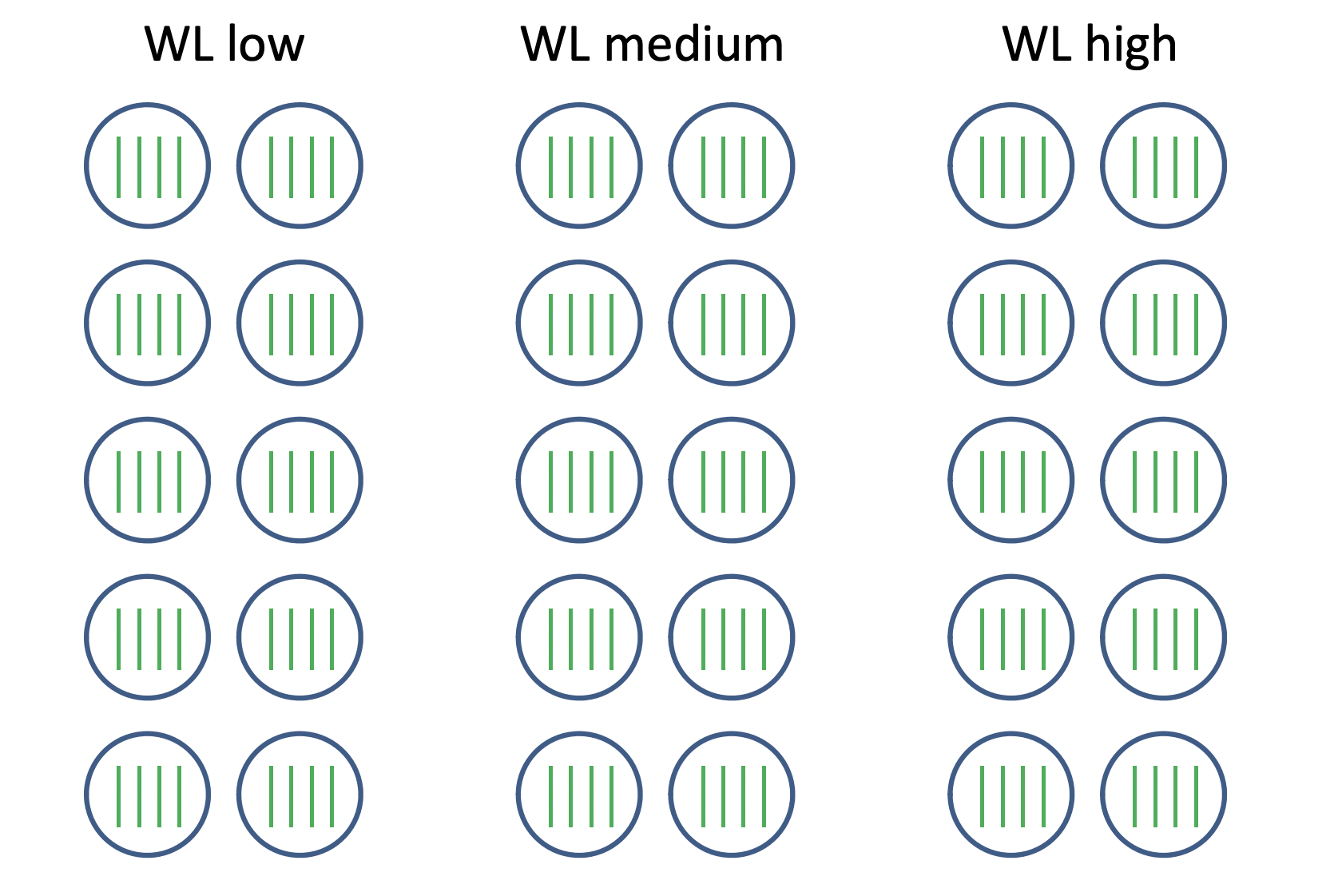
Researchers were interested in studying how soil moisture level affects the ability of plants to respond to a virus infection. A total of 30 pots were assigned to three watering levels (1 = low, 2 = medium, 3 = high) using a balanced and completely randomized design. Each of the 30 pots contained four seedlings. Two randomly selected seedlings within each pot were injected with a virus. The remaining two seedlings in each pot were “mock infected” by injection with a harmless substance. Two weeks after treatment, each seedling was individually weighed, and these weights served as the response variable for subsequent analysis.

Notation:
- \(i = 1, 2, 3\): watering levels
- \(j = 1, \ldots, 10\): pots within each watering levels
- \(k = 1, 2\) : infections (control, virus)
- \(l = 1, 2\): seedlings within watering level, pot, and infection
Model: \[ y_{ijkl} = \mu_{ik} + p_{ij} + e_{ijkl} \] where \(p_{ij} \sim N(0, \sigma_p^2)\), \(e_{ijkl} \sim N(0, \sigma_e^2)\).
ANOVA Table:

Source DF

wl 2

pot(wl) 27

inf 1

wl\(\times\) inf 2

error 87

c.total 119
SAS Code

Source	DF
wl	2
pot(wl)	27
inf	1
wl\(\times\) inf	2
error	87
c.total	119

  proc mixed; 
    class wl pot inf; 
    model y = wl inf wl*inf / ddfm = satterth; 
    random pot(wl); 
  run;

Example 2:

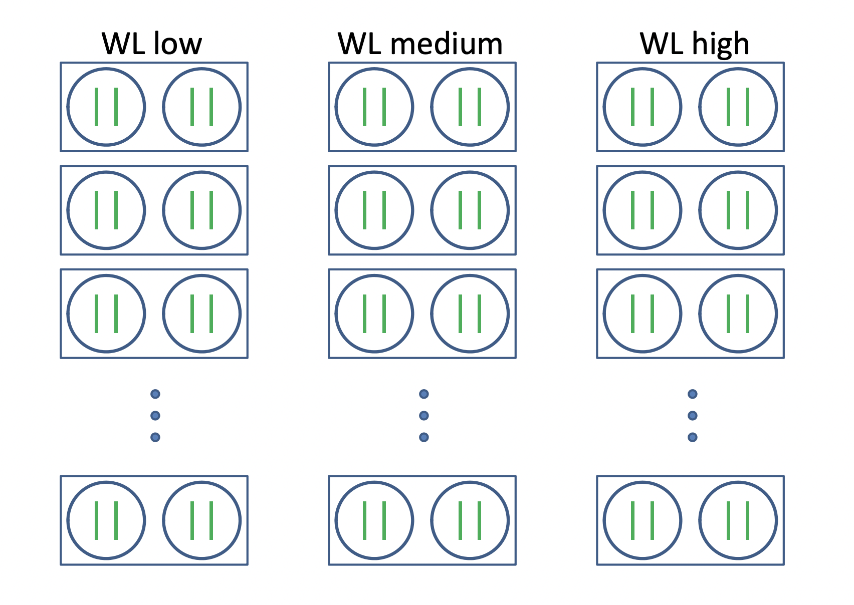
Researchers were interested in studying how soil moisture level affects the ability of plants to respond to a virus infection. A total of 30 trays were assigned to three watering levels (1 = low, 2 = medium, 3 = high) using a balanced and completely randomized design. Each of the 30 trays contained two pots. Each of the 60 pots contained two seedlings. The two seedlings in one randomly selected pot in each tray were injected with a virus. The two seedlings in the other pot on a given tray were “mock infected” by injection with a harmless substance. Two weeks after treatment, each seedling was individually weighed, and these weights served as the response variable for subsequent analysis.

Notation:
- \(i = 1, 2, 3\): watering levels
- \(j = 1, \ldots, 10\): trays within each watering level
- \(k = 1, 2\) : infections (control, virus)
- \(l = 1, 2\): seedlings within watering level, pot, and infection
Model: \[ y_{ijkl} = \mu_{ik} + t_{ij} + p_{ijk} + e_{ijkl} \] where \(t_{ij} \sim N(0, \sigma_t^2)\), \(p_{ijk} \sim N(0, \sigma_p^2)\), \(e_{ijkl} \sim N(0, \sigma_e^2)\).
ANOVA Table

Source DF

wl 2

tray(wl) 27

inf 1

wl\(\times\) inf 2

inf\(\times\)tray(wl) 27

error 60

c.total 119
SAS Code

Source	DF
wl	2
tray(wl)	27
inf	1
wl\(\times\) inf	2
inf\(\times\)tray(wl)	27
error	60
c.total	119

  proc mixed; 
    class wl tray inf; 
    model y = wl inf wl*inf/ ddfm = satterth; 
    random tray(wl) inf*tray(wl); 
  run;

Example 3:

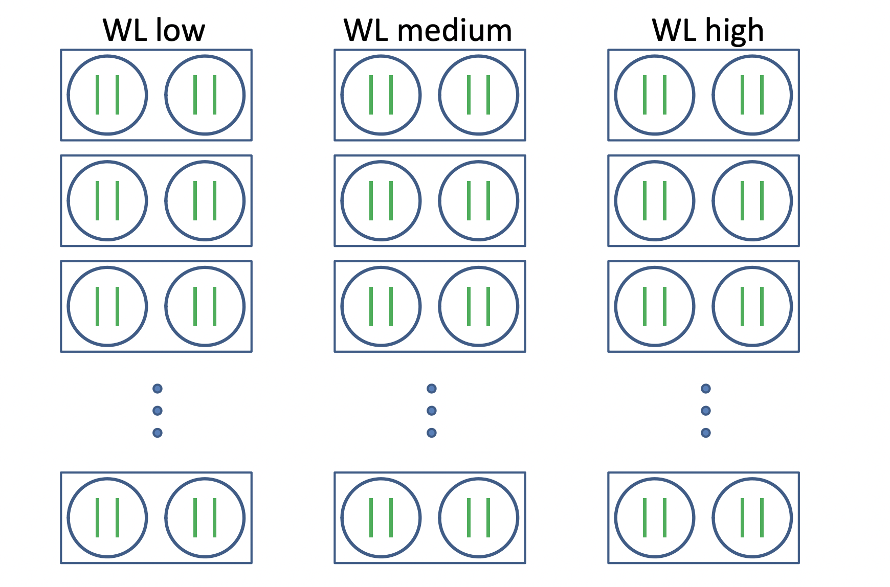
Researchers were interested in studying how soil moisture level affects the ability of plants to respond to a virus infection. A total of 30 trays were assigned to three watering levels (1 = low, 2 = medium, 3 = high) using a balanced and completely randomized design. Each of the 30 trays contained two pots. Each of the 60 pots contained two seedlings. In each pot, one of the two seedlings was randomly selected and injected with a virus; the other seedling in the pot was “mock infected” by injection with a harmless substance. Two weeks after treatment, each seedling was individually weighed, and these weights served as the response variable for subsequent analysis.

* Notation:

\(i = 1, 2, 3\): watering levels
\(j = 1, \ldots, 10\): trays within each watering level
\(k = 1, 2\) : pots within watering levels and trays
\(l = 1, 2\): infections (control, virus)
Model \[ y_{ijkl} = \mu_{ik} + t_{ij} + p_{ijk} + e_{ijkl} \]
ANOVA Table

Source DF

wl 2

tray(wl) 27

pot(wl tray) 30

inf 1

wl\(\times\)inf 2

error 57

c.total 119
SAS Code

Source	DF
wl	2
tray(wl)	27
pot(wl tray)	30
inf	1
wl\(\times\)inf	2
error	57
c.total	119

  proc mixed; 
    class wl tray pot inf; 
    model y = wl inf wl*inf / ddfm = satterth;
    random tray(wl) pot(wl tray); 
  run;

Example 4:

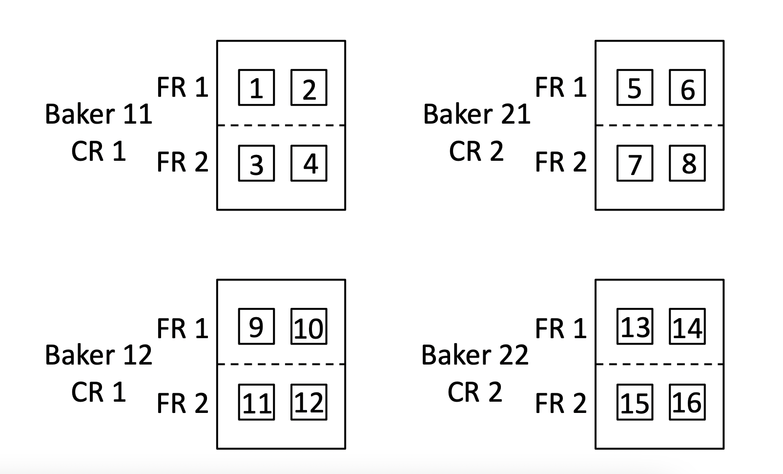
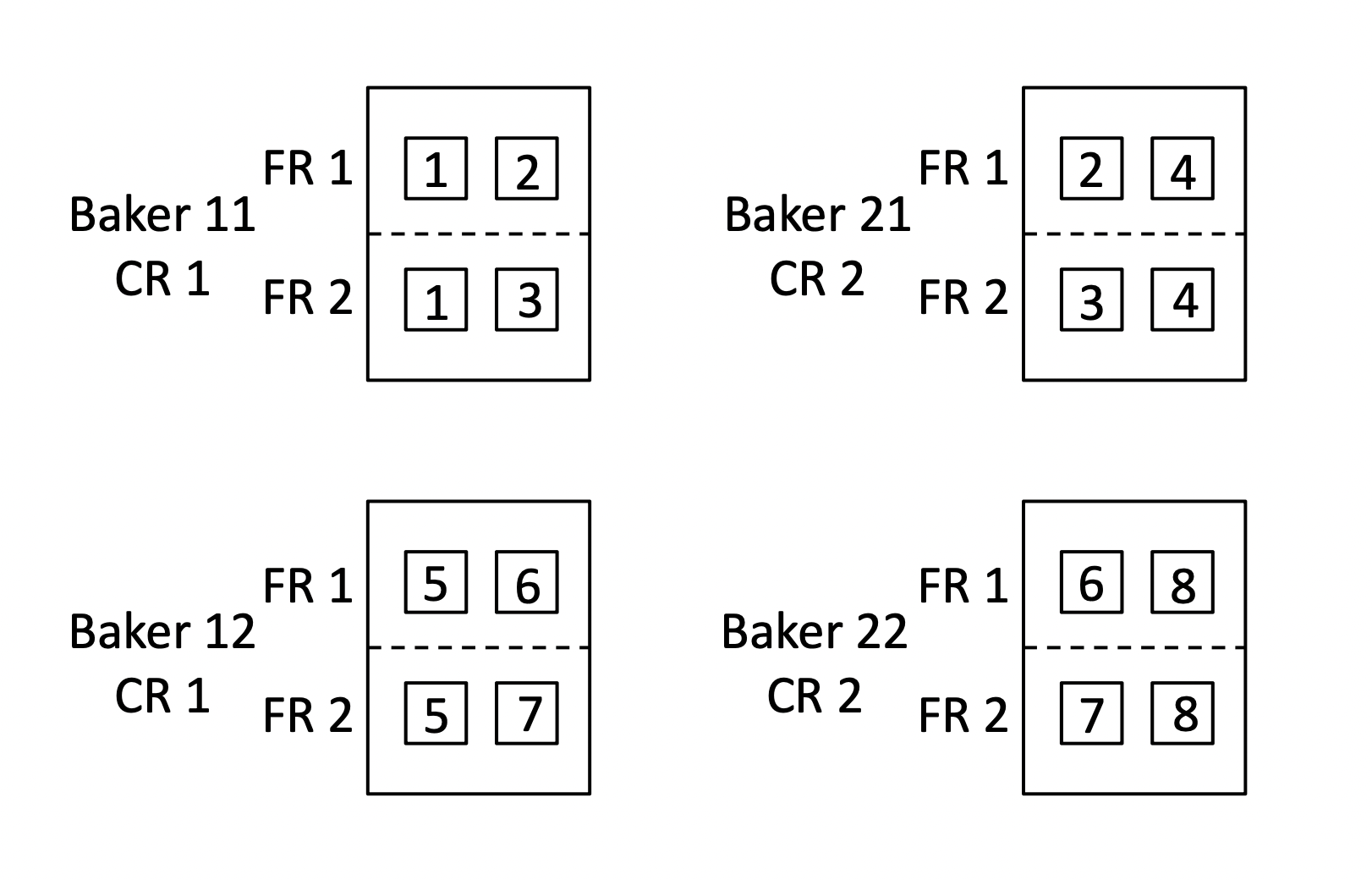
Researchers were interested in determining which combination of cake recipe and frosting recipe would yield the best tasting frosted cake. Two cake recipes (labeled CR1 and CR2) and two frosting recipes (labeled FR1 and FR2) were considered. The two cake recipes were randomly assigned to four bakers with two bakers for each cake recipe. Each baker prepared and baked a cake according to the recipe he or she was assigned. While cakes were baking and cooling, each baker prepared one batch of frosting using each of the frosting recipes. Half of each cake was randomly selected and covered with frosting prepared using FR1. The other half of each cake was covered with frosting prepared using FR2.

Two pieces of frosted cake from each half of each cake were scored for taste, with higher scores indicating better tasting frosted cake. The following diagram shows the four cakes baked by the four bakers as large rectangles. The dashed line on each rectangle shows the dividing point that separates FR1 frosting from FR2 frosting. The numbered squares within each rectangle show the pieces of frosted cake that were scored for taste.

Notation:
- \(i = 1, 2\): cake recipes
- \(j = 1, 2\): bakers within each cake recipe
- \(k = 1, 2\) : frosting recipes
- \(l = 1, 2\): pieces of cake within each half cake
Model \[ y_{ijkl} = \mu_{ik} + b_{ij} + h_{ijk} + e_{ijkl} \] where \(b_{11}, b_{12}, b_{21}, b_{22} \sim N(0, \sigma_{b}^2)\), \(h_{111}, \ldots, h_{222} \sim N(0, \sigma_h^2)\), \(e_{ijkl} \sim N(0, \sigma_e^2)\).
SAS Code

  proc mixed;
    class cr baker fr;
    model y=cr fr cr*fr / ddfm=satterth;
    random baker(cr) fr*baker(cr);
  run;

ANOVA Table

Source DF

cr 1

baker(cr) = whole plot error 2

fr 1

cr\(\times\)fr 1

fr\(\times\)baker(fr) 2

error = piece(cr, baker, fr) 8

c.total 15

Source	DF
cr	1
baker(cr) = whole plot error	2
fr	1
cr\(\times\)fr	1
fr\(\times\)baker(fr)	2
error = piece(cr, baker, fr)	8
c.total	15

Example 5:

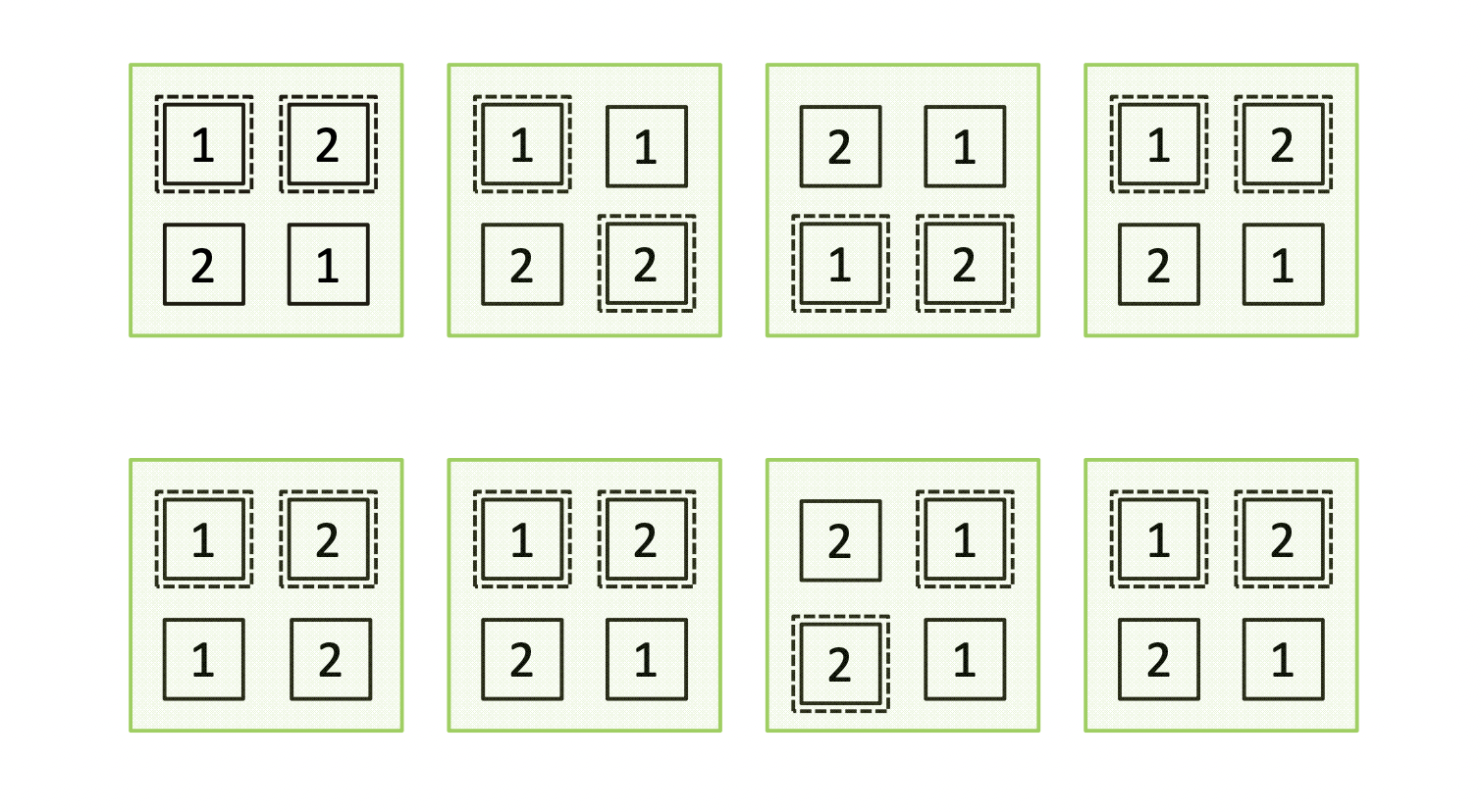
In the context of the frosted cake example (Example 4), a statistician is asked to analyze the data. The statistician asks, “How was the score for each piece of cake determined?”

Answer: Two pieces of frosted cake from each half of each cake were cut and delivered to eight trained judges for evaluation. Each judge tasted and separately assigned a score to two pieces of frosted cake. In the following diagram, the numbers 1 through 8 indicate the pieces of cake scored by judges 1 through 8, respectively.

Notation:
- \(i = 1, 2\): cake recipes
- \(j = 1, 2\): bakers within each cake recipe
- \(k = 1, 2\) : frosting recipes
- \(l = 1, 2\): pieces of cake within each half cake
Model \[ y_{ijkl} = \mu_{ik} + b_{ij} + h_{ijk} + t_l + e_{ijkl} \] where \(b_{11}, b_{12}, b_{21}, b_{22} \sim N(0, \sigma_{b}^2)\), \(h_{111}, \ldots, h_{222} \sim N(0, \sigma_h^2)\), \(t_1, \ldots, t_8 \sim N(0, \sigma_t^2)\), \(e_{ijkl} \sim N(0, \sigma_e^2)\).

SAS Code

proc mixed;
  class cr baker fr judge;
  model y=cr fr cr*fr / ddfm=satterth;
  random baker(cr) fr*baker(cr) judge;
  lsmeans cr fr cr*fr;
  estimate ...
run;

R Code

library(lme4)
library(lmerTest)
o = lmer(y ˜ cr + fr + cr:fr + (1 | baker) + (1 | baker:fr) + (1 | judge))
# cr %in% 1:2, fr %in% 1:2, baker %in% 1:4, judge %in% 1:8
anova(o)
ls_means(o)
contest(...)

ANOVA Table

Source DF

cr 1

baker(cr) 2

fr 1

cr\(\times\)fr 1

fr\(\times\)baker(fr) 2

judge 6

error 2

c.total 15

Source	DF
cr	1
baker(cr)	2
fr	1
cr\(\times\)fr	1
fr\(\times\)baker(fr)	2
judge	6
error	2
c.total	15

Example 6:

Researchers are interested in determining ways to deter deer from eating ornamental plants. An experiment was conducted in eight fields. Within each field, four 15 meter x 15 meter squares of land were studied. Within each field, researchers used the the following procedure:

Two of the four squares were randomly selected to be planted with plant type 1. The other two squares were planted with plant type 2.
One of the two squares planted with plant type 1 was randomly selected, and a fence was placed around the selected square. The other plant type 1 square was not surrounded by a fence.
One of the two squares planted with plant type 2 was randomly selected, and a fence was placed around the selected square. The other plant type 2 square was not surrounded by a fence.
Each of the four squares was divided into two rectangles of equal size. One rectangle within each square was randomly selected, and the plants growing in that rectangle were treated with a chemical. The other rectangle in each square was not treated with a chemical.
At the conclusion of the study, the amount of living plant biomass was measured for each rectangle.

Notation
- \(i = 1, 2\): plant types
- \(j = 1, 2\): fences (yes, no)
- \(k = 1, 2\) : chemicals (yes, no)
- \(l = 1, \ldots, 8\): fields
Model \[ y_{ijkl} = \mu_{ijk} + f_l + s_{ijl} + e_{ijkl} \] where \(f_l \sim N(0, \sigma_f^2)\), \(s_{ijl} \sim N(0, \sigma_s^2)\), \(e_{ijkl} \sim N(0, \sigma_e^2)\).

ANOVA Table

Source	DF	EMS
field	7	\(8\sigma_f^2 + 2\sigma_s^2 + \sigma_e^2\)
type	1
fence	1
ptype\(\times\)fence	1
field\(\times\)ptype+field\(\times\)fence+field\(\times\)ptype\(\times\)fence (whole plot error)	21	\(2\sigma_s^2 + \sigma_e^2\)
chem	1
ptype\(\times\)chem	1
fence\(\times\)chem	1
ptype\(\times\)fence\(\times\)chem	1
error = field\(\times\)chem+field\(\times\)ptype\(\times\)chem+field\(\times\)fence\(\times\)chem+field\(\times\)ptype\(\times\)fence\(\times\)chem (split-plot error)	28	\(\sigma_e^2\)
c.total	63

SAS Code

proc mixed;
  class field ptype fence chem;
  model y=ptype|fence|chem/ddfm=satterth;random field field*ptype*fence;
run;

Comment:

If a term like pot(tray) is specified, it should be the case that pots within each tray are replicates that are not treated differently within a tray

For example, pot(tray) is correct for Example 3 but not for Example 2

When levels of a factor B are different for each level of a factor A, we say that B is nested within A. In SAS, this is indicated by B(A). If C is nested within B, and B is nested within A, this is indicated by C(A B) in SAS. See nesting.sas for an example