Chapter 9 Orthogonal Linear Combinations, Contrasts and Additional Partitioning of ANOVA Sums of Squares

• Orthogonal: Under the model \(y = X\beta + \epsilon, \epsilon \sim N(0, \sigma^2 I)\), two estimable linear combinations \(c_1'\beta\) and \(c_2'\beta\) are orthogonal if and only if their BLUEs \(c_1'\hat\beta\) and \(c_2'\hat\beta\) are uncorrelated.

  • \(cov(c_1'\hat\beta, c_2\hat\beta) = \sigma^2 c_1'(X'X)^- c_2\). Thus, estimable linear combinations \(c_1'\beta\) and \(c_2'\beta\) are orthogonal if and only if \(c_1'(X'X)^-c_2 = 0\).

• Contrast: A linear combinations \(c'\beta\) is a contrast if and only if \(c'1 = 0.\)

• Orthogonal Contrast: Two estimable contrasts \(c'_1\beta\) and \(c_2'\beta\) are orthogonal are called orthogonal contrasts.

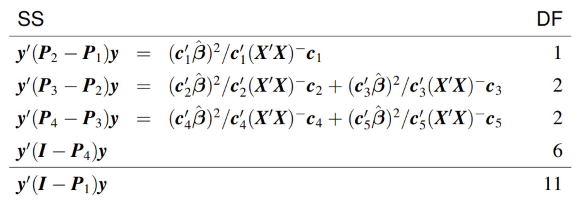
Suppose \(c_1'\beta, \ldots, c_q'\beta\) are pairwise orthogonal linear combinations. Let \(C' = [c_1, \ldots, c_q].\) When \(C\) has rank \(q\), \(\hat\beta'C'[C(X'X)^-C']^{-1}C\hat\beta = \sum_{i=1}^q (c_k'\hat\beta)^2/c_k'(X'X)^-c_k\).

• SAS code:

proc mixed;
    class diet drug;
    model weightgain=diet drug diet*drug;
    lsmeans diet*drug / slice=diet;
    estimate ’drug 1 - drug 2 for diet 1’  drug 1 -1 0 diet*drug 1 -1 0 0 0 0 / cl;
    estimate ’drug 1 - drug 3 for diet 1’  drug 1 0 -1 diet*drug 1 0 -1 0 0 0;
    estimate ’drug 2 - drug 3 for diet 1’  drug 0 1 -1 diet*drug 0 1 -1 0 0 0;
    estimate ’drug 1 - drug 2 for diet 2’  drug 1 -1 0 diet*drug 0 0 0 1 -1 0;
    estimate ’drug 1 - drug 3 for diet 2’  drug 1 0 -1 diet*drug 0 0 0 1 0 -1;
    estimate ’drug 2 - drug 3 for diet 2’  drug 0 1 -1 diet*drug 0 0 0 0 1 -1;
run;

• Comments on the analysis
  • Note that the main analysis focuses on pairwise comparisons of drugs within each diet.
  • This involves a set of six contrasts, but the contrasts are not pairwise orthogonal within either diet.
  • The sums of squares for these contrasts do not add up to any ANOVA sums of squares, but they are the contrasts that best address the researchers’ questions.
  • If we want to control the probability of one or more type I errors, we could use Bonferroni’s method. In this case, the adjustment for multiple testing would not change the conclusions.