Chapter 22 Additional Topics Related to Likelihood
Akaike’s Information Criteria: \(AIC = -2\ell(\hat\theta) + 2k\).
Schwarz’s Bayesian Information Criterion: \(BIC = -2\ell(\hat\theta) + k\ln n\)
If REML likelihoods are used, compared models must have the same model for the response mean. Different models for the mean would yield different error contrasts and different datasets for computation of maximized REML likelihoods.
Asymptotic normality of \(\hat\theta\): for sufficiently large \(n\), \(\hat\theta \stackrel{\cdot}{\sim} N(\theta, I^{-1}(\theta))\) where \(I(\theta) = \left[-E\{\frac{\partial^2 \ell(\theta)}{\partial \theta_i \partial \theta_j} \} \right]\) is called Fisher Information matrix.
- This implies \((\hat\theta - \theta)'[\widehat{Var}(\hat\theta)]^{-1}(\hat\theta - \theta) \stackrel{\cdot}{\sim}(\hat\theta - \theta) \stackrel{d}{\rightarrow} z'z \sim \chi_k^2\).
Wald Tests: Suppose for large \(n\) that \(\hat\theta \stackrel{\cdot}{\sim} N(\theta, \widehat{Var}(\hat\theta))\), then a confidence interval for \(c'\theta\) that has confidence level approximately equal to \(1 - \alpha\) is \(c'\hat\theta \pm z_{1-\alpha/2}\sqrt{c'\widehat{Var}(\hat\theta)c}\). Likewise, if \(C\) is a \(q \times k\) matrix of rank \(q\), a test of \(H_0: C\theta = d\) can be based on the test statistic \[ (C\hat\theta - d)'[C\widehat{Var}(\hat\theta)C']^{-1}(C\hat\theta - d) \sim \chi_q^2 \]
Multivarite Delta Method: Suppose a \(g\) is a function from \(R^k\) to \(R^m\), i.e. \(g = [g_1(\theta), \ldots, g_m(\theta)]'\). Let \(D \equiv \frac{\partial g}{\partial \theta}\) be the derivative matrix. By Taylor’s theorem, \(g(\hat\theta) \approx g(\theta) + D'(\hat\theta - \theta)\) which implies \(E(g(\hat\theta)) \approx g(\theta) + D'E(\hat\theta - \theta) = g(\theta)\) and \(Var(g(\hat\theta)) \approx Var[g(\theta) + D'(\hat\theta - \theta)] = D'Var(\hat\theta)D\). Therefore, \(g(\hat\theta) \stackrel{\cdot}{\sim} N(g(\theta), D'Var(\hat\theta) D)\).
Likelihood Ratio: Define \(\Lambda\) as \(\frac{\text{Reduced Model Maximial likelihood}}{\text{Full Model Maximized Likelihood}}\). \(-2\ln(\Lambda)\) is known as the likelihood ratio test statisti and \(-2\ln(\Lambda) \sim \chi_{k_f - k_r}^2\) under the null hypothesis.
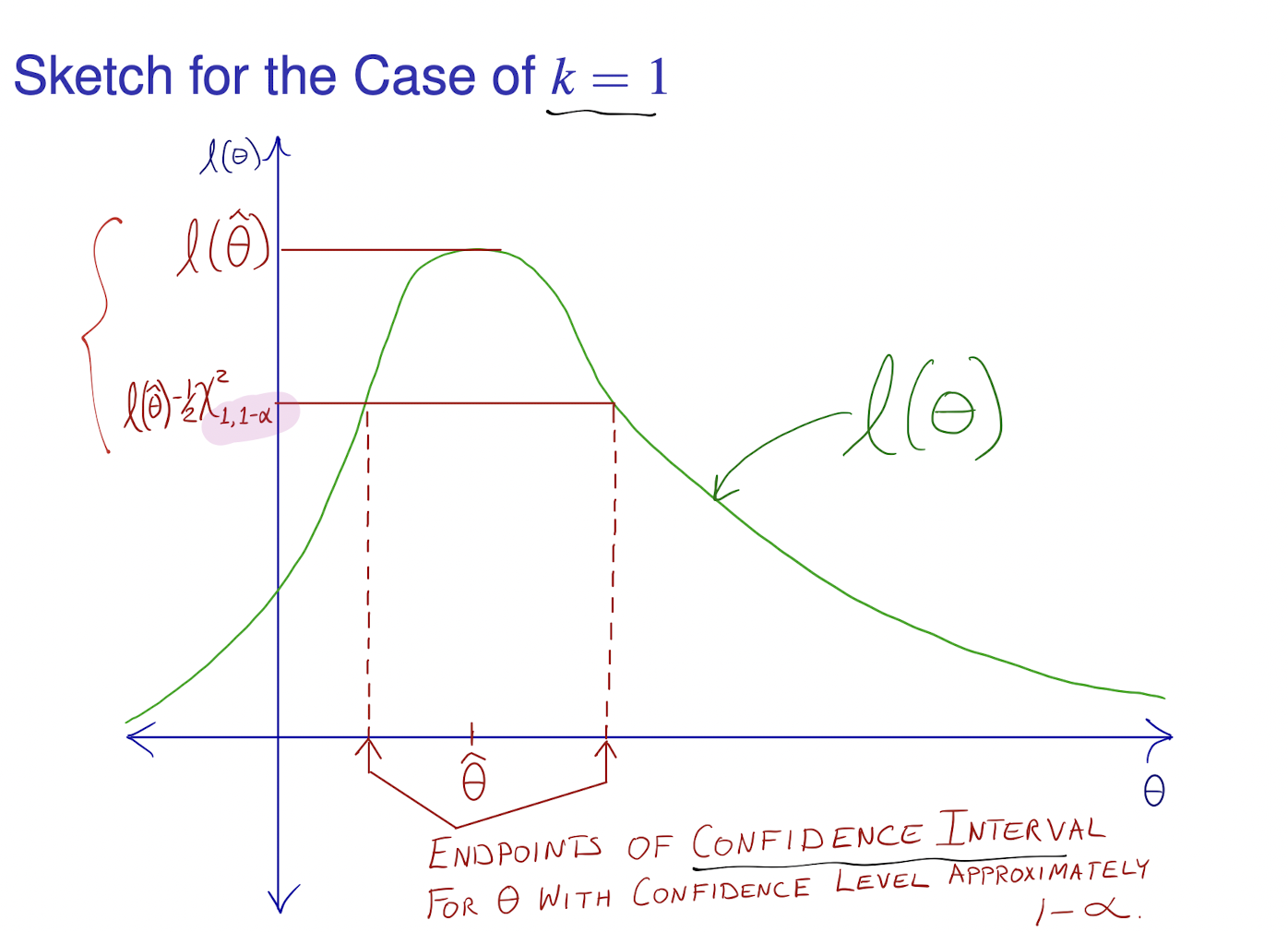
Profile Likelihood Confidence: \(\{\theta_1: \ell(\theta_1, \hat\theta_2(\theta_1)) \geq \ell(\hat\theta) - \frac{1}{2} \chi_{k_1, 1-\alpha}^2\}\).