Chapter 15 ANOVA for Balanced Split-Plot Experiments

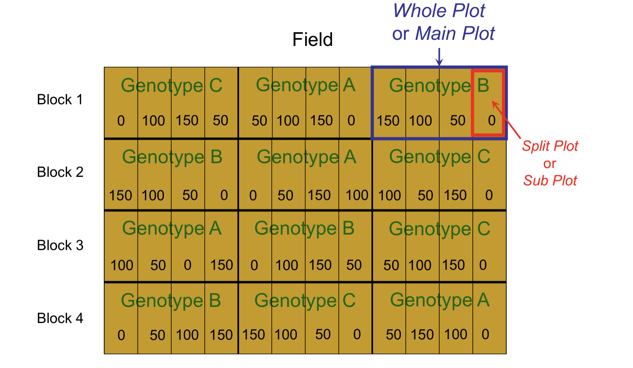
Model: \(y_{ijk} = \mu_{ij} + b_k + w_{ik} + e_{ijk}\), Genotype \(i = 1, 2, 3\), Fertilizer \(j = 1,2, 3,4\), Block \(k = 1, 2, 3, 4\).

• Because the experiment is balanced, the GLS estimator is equal to the OLS estimator for any estimable \(C\beta\): \(C\hat\beta_\Sigma = C\hat \beta\).

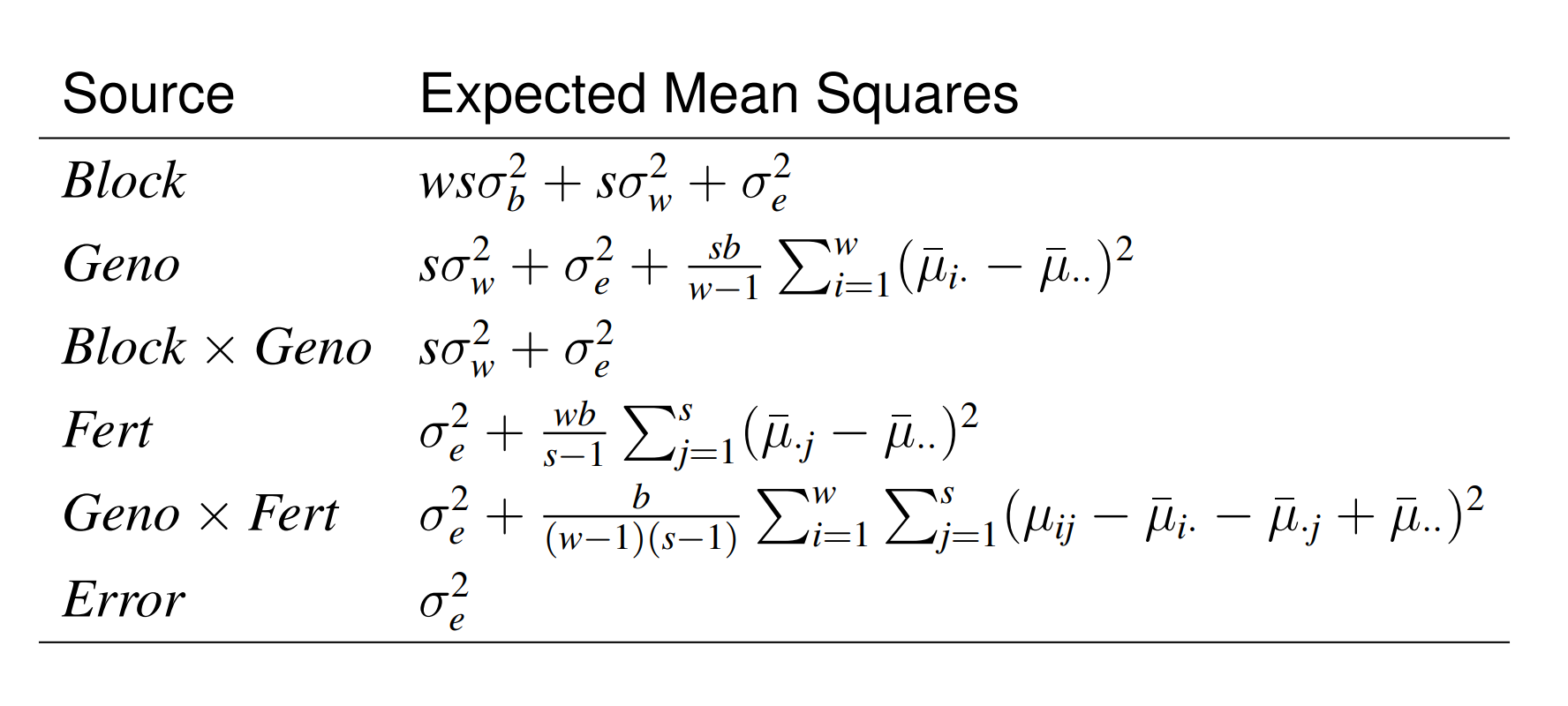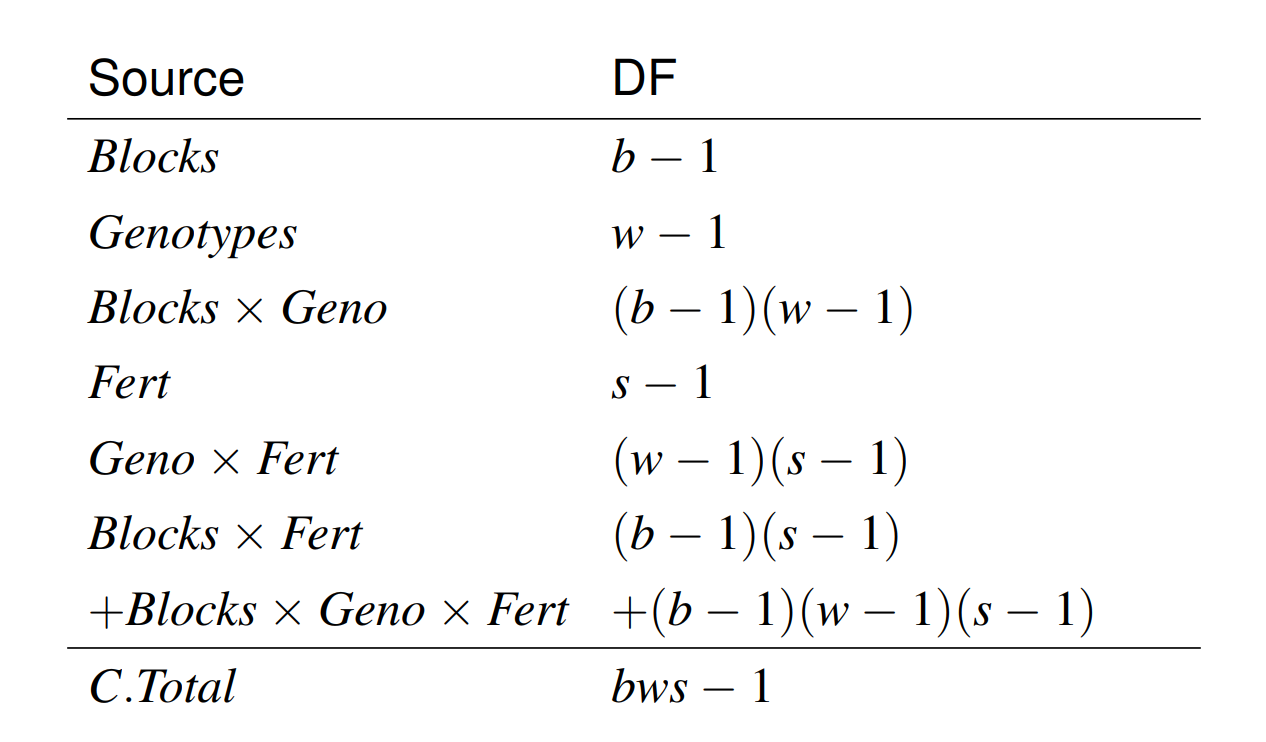
• there are no terms in our model corresponding to \(Block\times Fert\).

• \(E(MS_{Blocks\times Fert}) = E(MS_{Blocks\times Geno\times Fert}) = \sigma_e^2\).

  \[\begin{aligned}&E\left(M S_{\text {Geno }}\right)=\frac{s b}{w-1} \sum_{i=1}^{w} E\left(\bar{y}_{i . .}-\bar{y} \ldots\right)^{2} \\&\quad=\frac{s b}{w-1} \sum_{i=1}^{w} E\left(\bar{\mu}_{i}-\bar{\mu} . .+\bar{w}_{i}-\bar{w} . .+\bar{e}_{i .}-\bar{e} \ldots\right)^{2} \\&=s b\left\{\frac{\sum_{i=1}^{w}\left(\bar{\mu}_{i}-\bar{\mu} . .\right)^{2}}{w-1}+E\left[\frac{\sum_{i=1}^{w}\left(\bar{w}_{i}-\bar{w} . .\right)^{2}}{w-1}\right]+E\left[\frac{\sum_{i=1}^{w}\left(\bar{e}_{i . .}-\bar{e}_{\ldots} . .\right)^{2}}{w-1}\right]\right\} \\&=s b \frac{\sum_{i=1}^{w}\left(\bar{\mu}_{i}-\bar{\mu} . .\right)^{2}}{w-1}+s b \frac{\sigma_{w}^{2}}{b}+s b \frac{\sigma_{e}^{2}}{s b} \\&=s b \frac{\sum_{i=1}^{w}\left(\bar{\mu}_{i}-\bar{\mu} .\right)^{2}}{w-1}+s \sigma_{w}^{2}+\sigma_{e}^{2}\end{aligned}\]

  \[\begin{aligned}&E\left(M S_{\text {Block } \times \text { Geno }}\right)=\frac{s}{(w-1)(b-1)} \sum_{i=1}^{w} \sum_{k=1}^{b} E\left(\bar{y}_{i \cdot k}-\bar{y}_{i . .}-\bar{y}_{\cdot \cdot k}+\bar{y} \ldots\right)^{2} \\&=\frac{s}{(w-1)(b-1)} \sum_{i=1}^{w} \sum_{k=1}^{b} E\left(w_{i k}-\bar{w}_{i .}-\bar{w}_{\cdot k}+\bar{w}_{. .}+\bar{e}_{i \cdot k}-\bar{e}_{i . .}-\bar{e}_{. . k}+\bar{e}_{\ldots}\right)^{2} \\&=\frac{s}{(w-1)(b-1)} E\left[\sum_{i=1}^{w} \sum_{k=1}^{b}\left(w_{i k}-\bar{w}_{i} .\right)^{2}-2 \sum_{i=1}^{w} \sum_{k=1}^{b}\left(w_{i k}-\bar{w}_{i}\right)\left(\bar{w}_{\cdot k}-\bar{w} . .\right)\right. \\&\left.+\sum_{i=1}^{w} \sum_{k=1}^{b}\left(\bar{w}_{\cdot k}-\bar{w} . .\right)^{2}+e^{2} \text { sum }\right] \\&=\frac{s}{(w-1)(b-1)} E\left[\sum_{i=1}^{w} \sum_{k=1}^{b}\left(w_{i k}-\bar{w}_{i} .\right)^{2}-w \sum_{k=1}^{b}\left(\bar{w}_{\cdot k}-\bar{w} . .\right)^{2}+e^{2} \mathrm{sum}\right] \\&=\frac{s}{(w-1)(b-1)}\left[w(b-1) \sigma_{w}^{2}-w(b-1) \sigma_{w}^{2} / w+E\left(e^{2} \text { sum }\right)\right]\\ & = s\sigma_w^2 + \sigma_e^2\end{aligned}\]

  where

  \[ \begin{aligned}E\left(e^{2} \mathrm{sum}\right) &=E\left[\sum_{i=1}^{w} \sum_{k=1}^{b}\left(\bar{e}_{i \cdot k}-\bar{e}_{i .}-\bar{e}_{. . k}+\bar{e} \ldots\right)^{2}\right] \\&=\frac{(w-1)(b-1)}{s} \sigma_{e}^{2}\end{aligned}\]

Inference for Whole-Plot

• Test for whole-plot factor main effects:

  \[ H_0: \bar \mu_{1.} = \ldots = \bar\mu_{w.} \Leftrightarrow H_0: \frac{sb}{w-1}\sum_{i=1}^w (\bar \mu_{i.} - \bar \mu_{..})^2 = 0 \]

  We compare \(\frac{MS_{Geno}}{MS_{Block\times Geno}}\) to a central F-test with \(w- 1\) and \((w-1)(b-1)\) degrees of freedom.

• Comparison for whole-plot marginal means:

  \[ H_0: \bar \mu_{1.} = \bar \mu_{2.} \]

  Note that \[ \begin{aligned}\operatorname{Var}\left(\bar{y}_{1 . .}-\bar{y}_{2 . .}\right) &=\operatorname{Var}\left(\bar{\mu}_{1.}-\bar{\mu}_{2 .}+\bar{w}_{1.}-\bar{w}_{2 .}+\bar{e}_{1 . .}-\bar{e}_{2 \cdot .}\right) \\&=\frac{2 \sigma_{w}^{2}}{b}+\frac{2 \sigma_{e}^{2}}{s b} \\&=\frac{2}{s b}\left(s \sigma_{w}^{2}+\sigma_{e}^{2}\right)=\frac{2}{s b} E\left(M S_{B l o c k \times \text { Geno }}\right) \end{aligned} \]

  so that \(\widehat{\operatorname{Var}}\left(\bar{y}_{1..}-\bar{y}_{2..}\right)=\frac{2}{s b} M S_{B l o c k \times G e n o}\). We can use \[ t=\frac{\bar{y}_{1..}-\bar{y}_{2 ..}-\left(\bar{\mu}_{1.}-\bar{\mu}_{2.}\right)}{\sqrt{\frac{2}{s b} M S_{\text {Block } \times \text { Geno }}}} \sim t_{(w-1)(b-1)} \]

  to test \(H_0\).

• Multiple test for whole-plot marginal means: \[ H_{0}: \boldsymbol{C}\left[\begin{array}{c}\bar{\mu}_{1.} \\\vdots \\\bar{\mu}_{w.}\end{array}\right]=\mathbf{0}, \]

we can use an F statistics with \(q\) and \((w-1)(b-1)\) degrees of freedom: \[ F=\frac{\left(\boldsymbol{C}\left[\begin{array}{c}\bar{y}_{1..} \\\vdots \\\bar{y}_{w..}\end{array}\right]\right)^{\prime}\left[\frac{M S_{\text {Block } \times \text{Gen}}}{s b} \boldsymbol{C} \boldsymbol{C}^{\prime}\right]^{-1}\left(\boldsymbol{C}\left[\begin{array}{c}\bar{y}_{1..} \\\vdots \\\bar{y}_{w..}\end{array}\right]\right)}{q} \] where \(C\) is a matrix whose rows are contrast vectors so that \(C1= 0\).

Inference for Split-Plot

\[ \begin{aligned}E\left(M S_{F e r t}\right) &=\frac{w b}{s-1} \sum_{j=1}^{s} E\left(\bar{y}_{.j .}-\bar{y}_{...}\right)^{2} \\&=\frac{w b}{s-1} \sum_{j=1}^{s} E\left(\bar{\mu}_{. j}-\bar{\mu}_{..}+\bar{e}_{. j.}-\bar{e}_{...}\right)^{2} \\&=\frac{w b}{s-1} \sum_{j=1}^{s}\left(\bar{\mu}_{. j}-\bar{\mu}_{..}\right)^{2}+\sigma_{e}^{2} \\ E(MS_{error}) & = \sigma_e^2 \end{aligned} \]

• Test for split-plot main effects:

  \[H_{0}: \bar{\mu}_{.1}=\cdots=\bar{\mu}_{. s} \Longleftrightarrow H_{0}: \frac{w b}{s-1} \sum_{j=1}^{s}\left(\bar{\mu}_{. j}-\bar{\mu}_{..}\right)^{2}=0\]

  We compare \(\frac{MS_{Fert}}{MS_{error}}\) to a central F distribution with \(s-1\) and \(w(s-1)(b-1)\) degrees of freedom.

• Comparison for split-plot marginal means:

  \[ H_0: \bar \mu_{.1} = \bar \mu_{.2} \]

  We can use \[ t=\frac{\bar{y}_{.1.}-\bar{y}_{. 2 .}-\left(\bar{\mu}_{.1}-\bar{\mu}_{. 2}\right)}{\sqrt{\frac{2}{w b} M S_{E r r o r}}} \sim t_{w(s-1)(b-1)} \]

  because \(\operatorname{Var}\left(\bar{y}_{\cdot 1 \cdot}-\bar{y}_{\cdot 2 \cdot}\right) =\operatorname{Var}\left(\bar{\mu}_{\cdot 1}-\bar{\mu}_{\cdot 2}+\bar{e}_{\cdot 1 \cdot}-\bar{e}_{\cdot 2 \cdot}\right) =\frac{2}{w b} \sigma_{e}^{2}=\frac{2}{w b} E\left(M S_{\text {Error }}\right)\).

• Multiple test for split-plot marginal means: \[ H_{0}: \boldsymbol{C}\left[\begin{array}{c}\bar{\mu}_{.1} \\\vdots \\\bar{\mu}_{.w}\end{array}\right]=\mathbf{0}, \]

  we can use an F statistics with \(q\) and \(w(s-1)(b-1)\) degrees of freedom: \[ F=\frac{\left(\boldsymbol{C}\left[\begin{array}{c}\bar{y}_{.1.} \\\vdots \\\bar{y}_{.w.}\end{array}\right]\right)^{\prime}\left[\frac{M S_{Error}}{w b} \boldsymbol{C} \boldsymbol{C}^{\prime}\right]^{-1}\left(\boldsymbol{C}\left[\begin{array}{c}\bar{y}_{.1.} \\\vdots \\\bar{y}_{.1.}\end{array}\right]\right)}{q} \]

  where \(C\) is a matrix whose rows are contrast vectors so that \(C1= 0\).

Inference for Interactions

\[ \begin{aligned}&E\left(M S_{\text {Geno } \times \text { Fert }}\right)=\frac{b}{(w-1)(s-1)} \sum_{i=1}^{w} \sum_{j=1}^{s} E\left(\bar{y}_{i j.}-\bar{y}_{i ..}-\bar{y}_{.j.}+\bar{y}_{...}\right)^{2} \\&=\frac{b}{(w-1)(s-1)} \sum_{i=1}^{w} \sum_{j=1}^{s} E\left(\mu_{i j}-\bar{\mu}_{i.}-\bar{\mu}_{. j}+\bar{\mu}_{..}+\bar{e}_{i j .}-\bar{e}_{i . .}-\bar{e}_{.j .}+\bar{e}_{...}\right)^{2} \\&=\quad \cdots \\&=\frac{b}{(w-1)(s-1)} \sum_{i=1}^{w} \sum_{j=1}^{s}\left(\mu_{i j}-\bar{\mu}_{i.}-\bar{\mu}_{. j}+\bar{\mu}_{..}\right)^{2}+\sigma_{e}^{2}\end{aligned} \]

• Note that \(\mu_{i j}-\bar{\mu}_{i.}-\bar{\mu}_{. j}+\bar{\mu}_{..} = 0. \forall i, j\) is equivalent to \(\mu_{i j}-\bar{\mu}_{i^*j}-\bar{\mu}_{i j^*}+\bar{\mu}_{i^*j^*}, \forall i\neq i^*, j\neq j^*\). Therefore, \(\frac{b}{(w-1)(s-1)} \sum_{i=1}^{w} \sum_{j=1}^{s}\left(\mu_{i j}-\bar{\mu}_{i.}-\bar{\mu}_{. j}+\bar{\mu}_{..}\right)^{2} = 0\) can be used as null hypothesis for no interactions between genotypes and fertilizers.

• Test for Whole * Split interaction Effects

  \[ H_0: \frac{b}{(w-1)(s-1)} \sum_{i=1}^{w} \sum_{j=1}^{s}\left(\mu_{i j}-\bar{\mu}_{i.}-\bar{\mu}_{. j}+\bar{\mu}_{..}\right)^{2} = 0 \]

  We can compare \(\frac{MS_{Geno\times Fert}}{MS_{Error}}\) to a central F distribution with \((w-1)(s-1)\) and \(w(s-1)(b-1)\) degrees of freedom.

• Inference for simple effects:

  \[ H_0: \mu_{11} = \mu_{12} \]

  Note that \(\widehat{Var}(\bar y_{11.} -\bar y_{12.}) = \frac{2}{b}MS_{error}\), we can use \(t=\frac{\bar{y}_{11 \cdot}-\bar{y}_{12 \cdot}-\left(\mu_{11}-\mu_{12}\right)}{\sqrt{\frac{2}{b} M S_{\text {Error }}}} \sim t_{w(s-1)(b-1)}\) to test \(H_0\).

  However, \(Var(\bar y_{11.} - \bar y_{21.}) = \frac{2}{b}(\sigma_w^2 + \sigma_e^2)\) which is not a constant times any expected mean square from our ANOVA table. \(E(\frac{1}{s}MS_{Block\times Geno}+\frac{s-1}{s}MS_{error}) = \sigma_w^2 + \frac{\sigma_e^2}{s} + \frac{(s-1)\sigma_e^2}{s} = \sigma_w^2 + \sigma_e^2\). So that \(\widehat{Var}(\bar y_{11.} - \bar y_{21.})= \frac{2}{sb}MS_{Block\times Geno}+\frac{2s-2}{s}MS_{error}\). We can use

  \[ \frac{\bar{y}_{11 \cdot}-\bar{y}_{21 \cdot}-\left(\mu_{11}-\mu_{12}\right)}{\sqrt{\frac{2}{sb}MS_{Block\times Geno}+\frac{2s-2}{s}MS_{error}}} \sim t_{d} \text{ with }d \text{ degrees of freedom} \]

• Inference for Cell Means \(\mu_{ij}\): Note \(Var(\bar y_{ij.}) = \frac{\sigma_b^2}{b} + \frac{\sigma_w^2}{b} + \frac{\sigma_e^2}{b}\) so that we can construct unbiased estimator with approximate degrees of freedom from Cochran-Satterthwaite. ****