16 Single Index Model
Updated: October 16, 2020
Copyright © Eric Zivot 2015
Outline
- Single Index Model and Portfolio Theory
- portfolio optimization using SI covariance matrix
- always pd, reduces number of estimated components in matrix.
- Compare results with sample covariance matrix
- Risk analysis of asset and portfolios: factor risk reports
- portfolio optimization using SI covariance matrix
- Statistical Properties of Least Squares Estimates
- Bias
- Standard errors
- Asymptotic distributions and confidence intervals
- Hypothesis Testing in the Single Index Model
- Tests for coefficients
- Tests for model assumptions: check to see if residual correlation matrix is diagonal!
- Diagnostics for covariance stationarity
- Rolling estimates from the single index model
16.1 Motivation
The CER model for monthly asset returns assumes that returns are jointly normally distributed with a constant mean vector and covariance matrix. This model captures many of the stylized facts for monthly asset returns. While the CER model captures the covariances and correlations between different asset returns it does not explain where these covariances and correlations come from. The single index model is an extension of the CER model that explains the covariance and correlation structure among asset returns as resulting from common exposures to an underlying market index. The intuition behind the single index model can be illustrated by examining some example monthly returns.
For the single index model examples in this chapter, consider the monthly adjusted closing prices on four Northwest stocks (with tickers in parentheses): Boeing (BA), Nordstrom (JWN), Microsoft (MSFT), Starbucks (SBUX). We will also use the monthly adjusted closing prices on the S&P 500 index (^GSPC) as the proxy for the market index. These prices are extracted from the IntroCompFinR package as follows:
# get data from IntroCompFin package
data(baDailyPrices, jwnDailyPrices,
     msftDailyPrices, sbuxDailyPrices, sp500DailyPrices)
baPrices = to.monthly(baDailyPrices, OHLC=FALSE)
jwnPrices = to.monthly(jwnDailyPrices, OHLC=FALSE)
msftPrices = to.monthly(msftDailyPrices, OHLC=FALSE)
sbuxPrices = to.monthly(sbuxDailyPrices, OHLC=FALSE)
sp500Prices = to.monthly(sp500DailyPrices, OHLC=FALSE)
siPrices = merge(baPrices, jwnPrices, msftPrices,
                 sbuxPrices, sp500Prices)
The data sample is from January, 1998 through May, 2012 and returns are simple returns:
smpl = "1998-01::2012-05"
siPrices = siPrices[smpl]
siRetS = na.omit(Return.calculate(siPrices, method="simple"))
head(siRetS, n=3)
## BA JWN MSFT SBUX SP500
## Feb 1998 0.1425 0.1298 0.13640 0.0825 0.07045
## Mar 1998 -0.0393 0.1121 0.05570 0.1438 0.04995
## Apr 1998 -0.0396 0.0262 0.00691 0.0629 0.00908Prices are shown in Figure 16.1, created using:
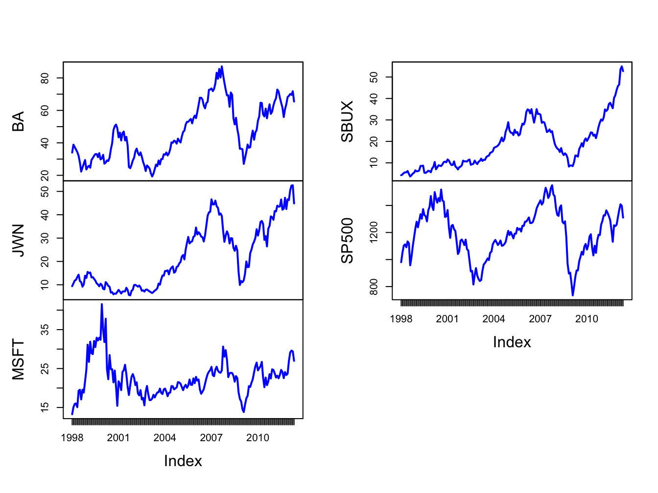
Figure 16.1: Monthly closing prices on four Northwest stocks and the S&P 500 index.
The time plots of prices show some common movements among the stocks that are similar to movements of the S&P 500 index . During the dot-com boom-bust at the beginning of the sample, except for Starbucks, prices rise during the boom and fall during the bust. For all assets, prices rise during the five year boom period prior to the financial crisis, fall sharply after 2008 during the bust, and then rise afterward.
Figure 16.2 shows time plots of the monthly returns on each stock together with the return on the S&P 500 index, created using
par(mfrow=c(2,2))
plot.zoo(siRetS[,c("SP500","BA")], plot.type="single",
         main="S&P 500 and Boeing", ylab="returns",
         col=c("blue","orange"), lwd=c(2,2))
abline(h=0)
plot.zoo(siRetS[,c("SP500","JWN")], plot.type="single",
         main="S&P 500 and Nordstom", ylab="returns",
         col=c("blue","orange"), lwd=c(2,2))
abline(h=0)
plot.zoo(siRetS[,c("SP500","MSFT")], plot.type="single",
         main="S&P 500 and Microsoft", ylab="returns",
         col=c("blue","orange"), lwd=c(2,2))
abline(h=0)
plot.zoo(siRetS[,c("SP500","SBUX")], plot.type="single",
         main="S&P 500 and Starbucks", ylab="returns",
         col=c("blue","orange"), lwd=c(2,2))
abline(h=0) 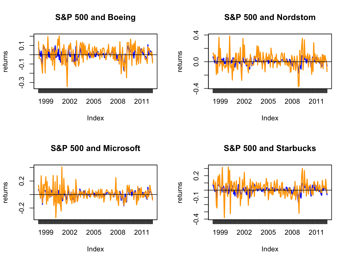
Figure 16.2: Monthly returns on four Northwest stocks. The orange line in each panel is the monthly return on the stock, and the blue line is the monthly return on the S&P 500 index.
Figure 16.2 shows that the individual stock returns are more volatile than the S&P 500 returns, and that the movement in stock returns (orange lines) tends to follow the movements in the S&P 500 returns indicating positive covariances and correlations.
The sample return covariance and correlation matrices are computed using:
##            BA     JWN    MSFT    SBUX   SP500
## BA    0.00796 0.00334 0.00119 0.00245 0.00223
## JWN   0.00334 0.01492 0.00421 0.00534 0.00339
## MSFT  0.00119 0.00421 0.01030 0.00348 0.00298
## SBUX  0.00245 0.00534 0.00348 0.01191 0.00241
## SP500 0.00223 0.00339 0.00298 0.00241 0.00228## BA JWN MSFT SBUX SP500
## BA 1.000 0.306 0.131 0.251 0.524
## JWN 0.306 1.000 0.340 0.401 0.581
## MSFT 0.131 0.340 1.000 0.314 0.614
## SBUX 0.251 0.401 0.314 1.000 0.463
## SP500 0.524 0.581 0.614 0.463 1.000The sample correlation matrix is visualized in Figure 16.3
using the corrplot function corrplot.mixed():
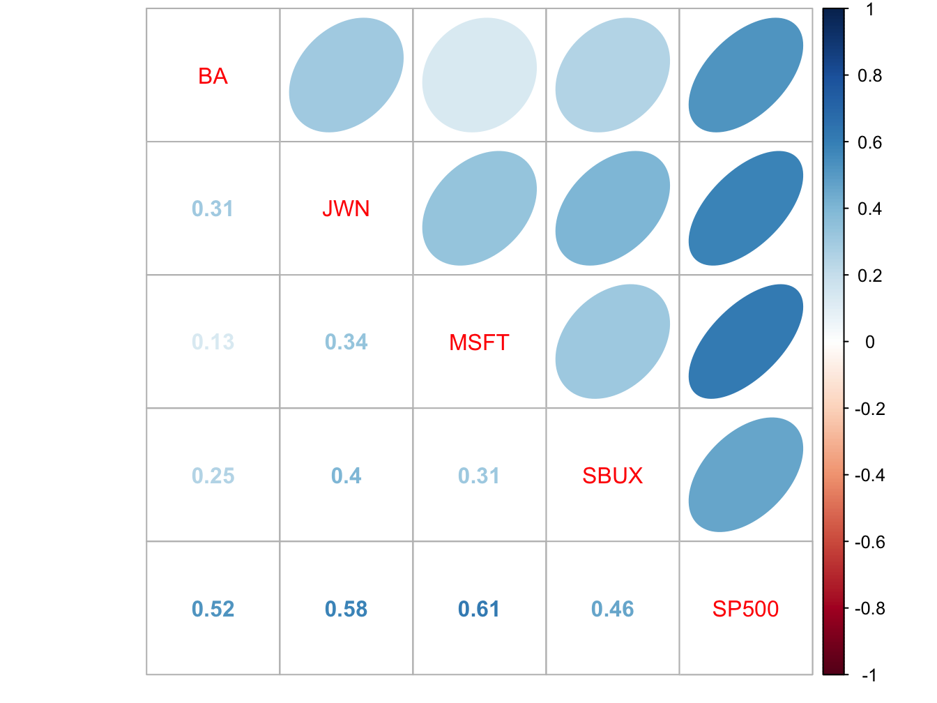
Figure 16.3: Sample correlation matrix of monthly returns.
All returns are positively correlated and each stock return has the highest positive correlation with the S&P 500 index.
The positive covariance and correlation of each stock return with the market return can also be visualized with scatterplots as illustrated in Figure 16.4, created with:
siRetSmat = coredata(siRetS)
par(mfrow=c(2,2))
plot(siRetSmat[, "SP500"], siRetSmat[, "BA"],
     main="S&P 500 and Boeing", col="cornflowerblue",
     lwd=2, pch=16, cex=2, xlab="S&P 500",
     ylab="BA", ylim=c(-0.4, 0.4))
abline(h=0,v=0)
plot(siRetSmat[, "SP500"], siRetSmat[, "JWN"],
     main="S&P 500 and Nordstrom", col="cornflowerblue",
     lwd=2, pch=16, cex=2, xlab="S&P 500",
     ylab="JWN", ylim=c(-0.4, 0.4))
abline(h=0,v=0)
plot(siRetSmat[, "SP500"], siRetSmat[, "MSFT"],
     main="S&P 500 and Microsoft", col="cornflowerblue",
     lwd=2, pch=16, cex=2, xlab="S&P 500",
     ylab="MSFT", ylim=c(-0.4, 0.4))
abline(h=0,v=0)
plot(siRetSmat[, "SP500"], siRetSmat[, "SBUX"],
     main="S&P 500 and Starbucks", col="cornflowerblue",
     lwd=2, pch=16, cex=2, xlab="S&P 500",
     ylab="SBUX", ylim=c(-0.4, 0.4))
abline(h=0,v=0)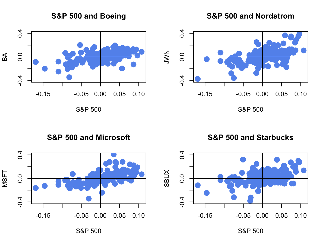
Figure 16.4: Monthly return scatterplots of each stock vs. the S&P 500 index.
The scatterplots show that as the market return increases, the returns on each stock increase in a linear way.
\(\blacksquare\)
16.2 William Sharpe’s SI Model
- What is SI model used for? Extension of the CER model to capture the stylized fact of a common component in the returns of many assets.
- Provides an explanation as to why assets are correlated with each other: share an exposure to a common source.
- Provides a simplification of the covariance matrix of a large number of asset returns.
- Provides additional intuition about risk reduction through diversification.
- Example of a factor model for asset returns. Factor models are used heavily in academic theories of asset pricing and in industry for explaining asset returns, portfolio construction and risk analysis. Sharpe’s SI model is the most widely used.
- Motivate by showing positive correlation between individual asset returns and market index (sp500)
- Mostly used for simple returns; but can be used for cc returns for risk analysis.
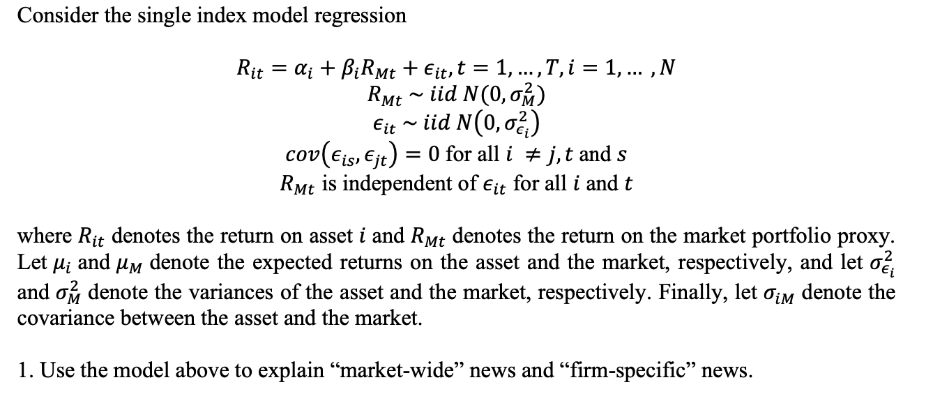
Let \(R_{it}\) denote the simple return on asset \(i\) over the investment horizon between times \(t-1\) and \(t\). Let \(R_{Mt}\) denote the simple return on a well diversified market index portfolio, such as the S&P 500 index. The single index (SI) model for \(R_{it}\) has the form:96 \[\begin{eqnarray} R_{it} & = & \alpha_{i}+\beta_{i}R_{Mt}+\varepsilon_{it},\tag{16.1}\\ R_{Mt} & \sim & iid\,N(0,\sigma_{M}^{2}),\tag{16.2}\\ \epsilon_{it} & \sim & \mathrm{GWN}\,(0,\sigma_{\epsilon,i}^{2}),\tag{16.3}\\ \mathrm{cov}(R_{Mt},\epsilon_{is}) & = & 0,\,\mathrm{f}\mathrm{or\,all}\,t\,\mathrm{and}\,s,\tag{16.4}\\ \mathrm{cov}(\epsilon_{it},\epsilon_{js}) & = & 0,\,\mathrm{for\,all}\,i\neq j\,\mathrm{and\,all}\,t\,\mathrm{and}\,s.\tag{16.5} \end{eqnarray}\] The SI model (16.1) - (16.5) assumes that all individual asset returns, \(R_{it},\) are covariance stationary and are a linear function of the market index return, \(R_{Mt},\) and an independent error term, \(\epsilon_{it}.\) The SI model is an important extension of the regression form of the CER model. In the SI model individual asset returns are explained by two distinct sources: (1) a common (to all assets) market-wide source \(R_{Mt}\); (2) and asset specific source \(\epsilon_{it}\).
16.2.1 Economic interpretation of the SI model
16.2.1.1 Interpretation of \(\beta_{i}\)
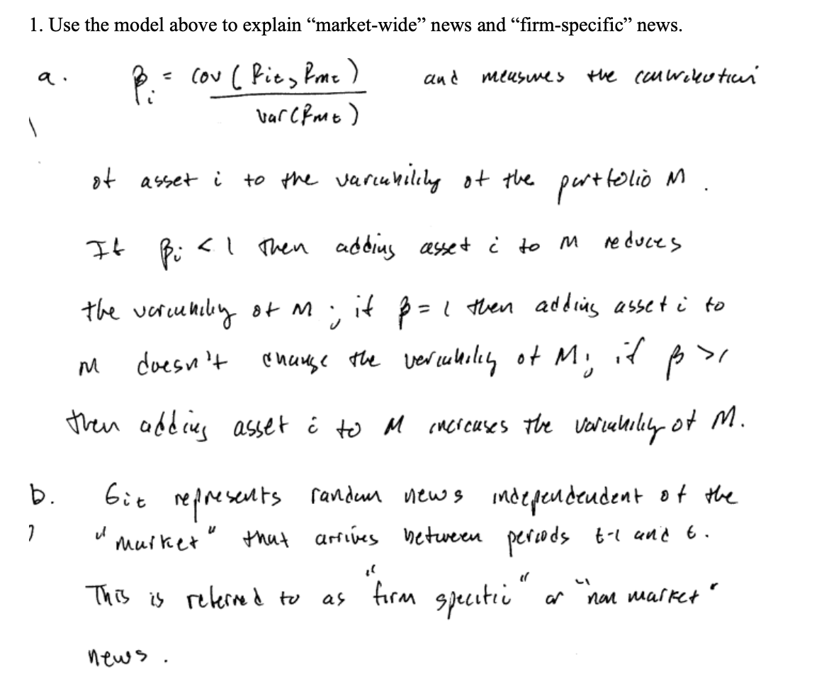
First, consider the interpretation of \(\beta_{i}\) in (16.1). The coefficient \(\beta_{i}\) is called the asset’s market exposure or market “beta”{Market beta}. It represents the slope coefficient in the linear relationship between \(R_{it}\) and \(R_{Mt}\). Because it is assumed that \(R_{Mt}\) and \(\epsilon_{it}\) are independent, \(\beta_{i}\) can be interpreted as the partial derivative \[ \frac{\partial R_{it}}{\partial R_{Mt}}=\frac{\partial}{\partial R_{Mt}}(\alpha_{i}+\beta_{i}R_{Mt}+\varepsilon_{it})=\beta_{i}. \] Then, for small changes in \(R_{Mt}\) denoted \(\Delta R_{Mt}\) and holding \(\varepsilon_{it}\) fixed, we have the approximation \[ \frac{\Delta R_{it}}{\Delta R_{Mt}}\approx\beta_{i}\Rightarrow\Delta R_{it}\approx\beta_{i}\times\Delta R_{Mt}, \] Hence, for a given change in the market return \(\beta_{i}\) determines the magnitude of the response of asset \(i's\) return. The larger (smaller) is \(\beta_{i}\) the larger (smaller) is the response of asset \(i\) to the movement in the market return.
The coefficient \(\beta_{i}\) in (16.1) has another interpretation that is directly related to portfolio risk budgeting. In particular, from chapter 14 \[\begin{equation} \beta_{i}=\frac{\mathrm{cov}(R_{it},R_{Mt})}{\mathrm{var}(R_{Mt})}=\frac{\sigma_{iM}}{\sigma_{M}^{2}},\tag{16.6} \end{equation}\] and \[ \mathrm{MC}\mathrm{R}_{i}^{\sigma_{M}}=\beta_{i}\sigma_{M}. \] Here, we see that \(\beta_{i}\) is the “beta” of asset \(i\) with respect to the market portfolio and so it is proportional to the marginal contribution of asset \(i\) to the volatility of the market portfolio. Therefore, assets with large (small) values of \(\beta_{i}\) have large (small) contributions to the volatility of the market portfolio. In this regard, \(\beta_{i}\) can be thought of as a measure of portfolio risk. Increasing allocations to assets with high (low) \(\beta_{i}\) values will increase (decrease) portfolio risk (as measured by portfolio volatility). In particular, when \(\beta_{i}=1\) asset \(i's\) percent contribution to the volatility of the market portfolio is its allocation weight. When \(\beta_{i}>1\) asset \(i's\) percent contribution to the volatility of the market portfolio is greater than its allocation weight, and when \(\beta_{i}<1\) asset \(i's\) percent contribution to the volatility of the market portfolio is less than its allocation weight.
The derivation of (16.6) is straightforward. Using (16.1) we can write \[\begin{align*} \mathrm{cov}(R_{it},R_{Mt}) & =\mathrm{cov}(\alpha_{i}+\beta_{i}R_{Mt}+\varepsilon_{it},R_{Mt})\\ & =\mathrm{cov}(\beta_{i}R_{Mt},R_{Mt})+\mathrm{cov}(\varepsilon_{it},R_{Mt})\\ & =\beta_{i}\mathrm{var}(R_{Mt})\text{ }\ (\text{since }\mathrm{cov}(\varepsilon_{it},R_{Mt})=0)\\ & \Rightarrow\beta_{i}=\frac{\mathrm{cov}(R_{it},R_{Mt})}{\mathrm{var}(R_{Mt})}. \end{align*}\]
16.2.1.2 Interpretation of \(R_{Mt}\) and \(\epsilon_{it}\)
To aid in the interpretation of \(R_{Mt}\) and \(\epsilon_{it}\) in (16.1) , re-write (16.3) as \[\begin{equation} \varepsilon_{it}=R_{it}-\alpha_{i}-\beta_{i}R_{Mt}.\tag{16.7} \end{equation}\] In (16.3), we see that \(\epsilon_{it}\) is the difference between asset \(i's\) return, \(R_{it},\) and the portion of asset \(i's\) return that is explained by the market return, \(\beta_{i}R_{Mt}\), and the intercept, \(\alpha_{i}.\) We can think of \(R_{Mt}\) as capturing “market-wide” news at time \(t\) that is common to all assets, and \(\beta_{i}\) captures the sensitivity or exposure of asset \(i\) to this market-wide news. An example of market-wide news is the release of information by the government about the national unemployment rate. If the news is good then we might expect \(R_{Mt}\) to increase because general business conditions are good. Different assets will respond differently to this news and this differential impact is captured by \(\beta_{i}.\) Assets with positive values of \(\beta_{i}\) will see their returns increase because of good market-wide news, and assets with negative values of \(\beta_{i}\) will see their returns decrease because of this good news. Hence, the magnitude and direction of correlation between asset returns can be partially explained by their exposures to common market-wide news. Because \(\epsilon_{it}\) is assumed to be independent of \(R_{Mt}\) and of \(\epsilon_{jt}\), we can think of \(\epsilon_{it}\) as capturing specific news to asset \(i\) that is unrelated to market news or to specific news to any other asset \(j\). Examples of asset-specific news are company earnings reports and reports about corporate restructuring (e.g., CEO resigning). Hence, specific news for asset \(i\) only effects the return on asset \(i\) and not the return on any other asset \(j\).
The CER model does not distinguish between overall market and asset specific news and so allows the unexpected news shocks \(\epsilon_{it}\) to be correlated across assets. Some news is common to all assets but some is specific to a given asset and the CER model error includes both types of news. In this regard, the CER model for an asset’s return is not a special case of the SI model when \(\beta_{i}=0\) because the SI model assumes that \(\epsilon_{it}\) is uncorrelated across assets.
16.2.2 Statistical properties of returns in the SI model
In this sub-section we present and derive the statistical properties of returns in the SI model (16.1) - (16.5). We will derive two types of statistical properties: unconditional and conditional. The unconditional properties are based on unconditional or marginal distribution of returns. The conditional properties are based on the distribution of returns conditional on the value of the market return.
16.2.2.1 Unconditional properties
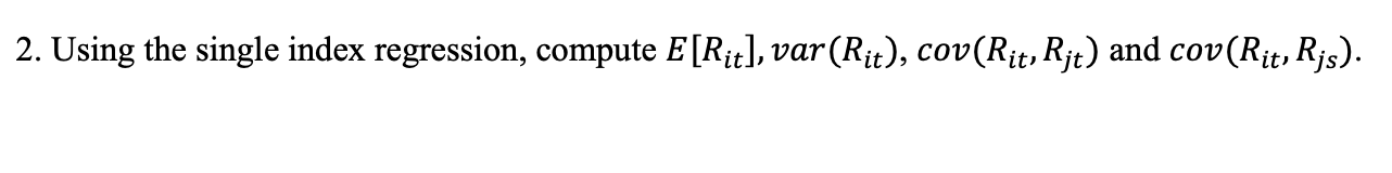
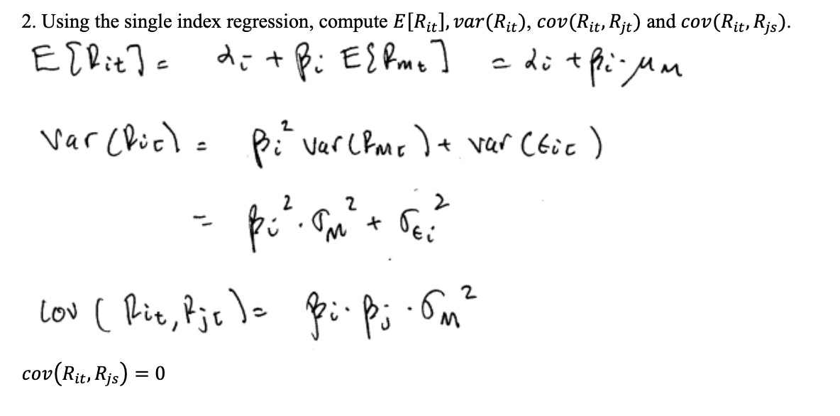
The unconditional properties of returns in the SI model (16.1) - (16.5) are: \[\begin{eqnarray} E[R_{it}] & = & \mu_{i}=\alpha_{i}+\beta_{i}\mu_{M},\tag{16.8}\\ \mathrm{var}(R_{it}) & = & \sigma_{i}^{2}=\beta_{i}^{2}\sigma_{M}^{2}+\sigma_{\epsilon,i}^{2},\tag{16.9}\\ \mathrm{cov}(R_{it},R_{jt}) & = & \sigma_{ij}=\beta_{i}\beta_{j}\sigma_{M}^{2},\tag{16.10}\\ \mathrm{cor}(R_{it},R_{jt}) & = & \rho_{ij}=\frac{\beta_{i}\beta_{j}\sigma_{M}^{2}}{\sqrt{(\beta_{i}^{2}\sigma_{M}^{2}+\sigma_{\epsilon,i}^{2})(\beta_{j}^{2}\sigma_{M}^{2}+\sigma_{\epsilon,j}^{2})}},\tag{16.11}\\ R_{it} & \sim & iid\,N(\mu_{i},\sigma_{i}^{2})=N(\alpha_{i}+\beta_{i}\mu_{M},\beta_{i}^{2}\sigma_{M}^{2}+\sigma_{\epsilon,i}^{2})\tag{16.12} \end{eqnarray}\] The derivations of these properties are straightforward and are left as end-of-chapter exercises.
Property (16.8) shows that \[\begin{equation} \alpha_{i}=\mu_{i}-\beta_{i}\mu_{M}.\tag{16.13} \end{equation}\] Hence, the intercept term \(\alpha_{i}\) can be interpreted as the average return on asset \(i\) that is in excess of the average return due to the market.
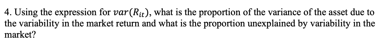
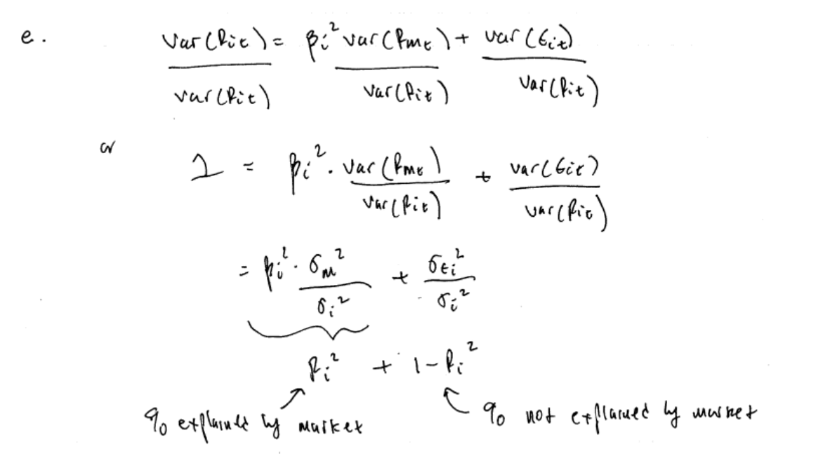
From property (16.9), an asset’s return variance is additively decomposed into two independent components: \[\begin{eqnarray} \mathrm{var}(R_{it}) & = & \sigma_{i}^{2}=\beta_{i}^{2}\sigma_{M}^{2}+\sigma_{\epsilon,i}^{2}\tag{16.14}\\ \mathrm{(total\,asset\,}i\,\mathrm{variance} & = & \mathrm{market\,variance}+\mathrm{asset\,specific\,variance)}\nonumber \end{eqnarray}\] Here, \(\beta_{i}^{2}\sigma_{M}^{2}\) is the contribution of the market index return \(R_{Mt}\) to the total variance of asset \(i\), and \(\sigma_{\epsilon,i}^{2}\) is the contribution of the asset specific component \(\epsilon_{it}\) to the total return variance, respectively. If we divide both sides of (16.14) by \(\sigma_{i}^{2}\) we get \[\begin{eqnarray*} 1 & = & \frac{\beta_{i}^{2}\sigma_{M}^{2}}{\sigma_{i}^{2}}+\frac{\sigma_{\epsilon,i}^{2}}{\sigma_{i}^{2}}\\ & = & R+(1-R^{2}), \end{eqnarray*}\] where \[\begin{equation} R^{2}=\frac{\beta_{i}^{2}\sigma_{M}^{2}}{\sigma_{i}^{2}}\tag{16.15} \end{equation}\] is the proportion of asset \(i's\) variance that is explained by the variability of the market return \(R_{Mt}\) and \[\begin{equation} 1-R^{2}=\frac{\sigma_{\epsilon,i}^{2}}{\sigma_{i}^{2}}\tag{16.16} \end{equation}\] is the proportion of asset \(i's\) variance that is explained by the variability of the asset specific component \(\epsilon_{it}.\)
- Sharpe’s rule of thumb. A typical stock has \(R^{2}=0.30\). That is, 30% of an asset’s variability is explained by the market movements. - \(R^{2}\) can be interpreted as the fraction of risk that is non-diversifiable, \(1-R^{2}\) gives the fraction of risk that is diversifiable. Come back to this point after discussing the SI model and portfolios below.
- This is an example of factor risk budgeting
Properties (16.10) and (16.11) show how assets are correlated in the SI model. In particular,
- \(\sigma_{ij}=0\) if \(\beta_{i}=0\) or \(\beta_{j}=0\) or both. Assets \(i\) and \(j\) are uncorrelated if asset \(i\) or asset \(j\) or both do not respond to market news.
- \(\sigma_{ij}>0\) if \(\beta_{i},\beta_{j}>0\) or \(\beta_{i},\beta_{j}<0\) . Assets \(i\) and \(j\) are positively correlated if both assets respond to market news in the same direction.
- \(\sigma_{ij}<0\) if \(\beta_{i}>0\) and \(\beta_{j}<0\) or if \(\beta_{i}<0\) and \(\beta_{j}>0\). Assets \(i\) and \(j\) are negatively correlated if they respond to market news in opposite directions.
From (16.11), assets \(i\) and \(j\) are perfectly correlated (\(\rho_{ij}=\pm1)\) only if \(\sigma_{\epsilon,i}=\sigma_{\epsilon,j}=0\).
Property (16.12) shows that the distribution of asset returns in the SI model is normal with mean and variance given by () and (), respectively.
In summary, the unconditional properties of returns in the SI model are similar to the properties of returns in the CER model: Returns are covariance stationary with constant means, variances, and covariances. Returns on different assets can be contemporaneously correlated and all asset returns uncorrelated over time. The SI model puts more structure on the expected returns, variances and covariances than the CER model and this allows for a deeper understanding of the behavior of asset returns.
16.2.2.2 Conditional properties
The properties of returns in the SI model (16.1) - (16.5) conditional on \(R_{Mt}=r_{Mt}\) are: \[\begin{eqnarray} E[R_{it}|R_{Mt} & = & r_{Mt}]=\alpha_{i}+\beta_{i}r_{Mt},\\ \mathrm{var}(R_{it}|R_{Mt} & = & r_{Mt}]=\sigma_{\epsilon,i}^{2},\\ \mathrm{cov}(R_{it},R_{jt}|R_{Mt} & = & r_{Mt}]=0,\\ \mathrm{cor}(R_{it},R_{jt}|R_{Mt} & = & r_{Mt}]=0,\\ R_{it}|R_{Mt} & \sim & iid\,N(\alpha_{i}+\beta_{i}r_{Mt},\sigma_{\epsilon,i}^{2}). \end{eqnarray}\]
Recall, conditioning on a random variable means we observe its value. In the SI model, once we observe the market return two important things happen: (1) an asset’s return variance reduces to its asset specific variance; and (2) asset returns become uncorrelated.
16.2.3 SI model and portfolios
A nice feature of the SI model for asset returns is that it also holds for a portfolio of asset returns. This property follows because asset returns are a linear function of the market return. To illustrate, consider a two asset portfolio with investment weights \(x_{1}\)and \(x_{2}\) where each asset return is explained by the SI model: \[\begin{eqnarray*} R_{1t} & = & \alpha_{1}+\beta_{1}R_{Mt}+\epsilon_{1t},\\ R_{2t} & = & \alpha_{2}+\beta_{2}R_{Mt}+\epsilon_{2t}. \end{eqnarray*}\] Then the portfolio return is \[\begin{align*} R_{p,t} & =x_{1}R_{1t}+x_{2}R_{2t}\\ & =x_{1}(\alpha_{1}+\beta_{1}R_{Mt}+\varepsilon_{1t})+x_{2}(\alpha_{2}+\beta_{2}R_{Mt}+\varepsilon_{2t})\\ & =\left(x_{1}\alpha_{1}+x_{2}\alpha_{2}\right)+\left(x_{1}\beta_{1}+x_{2}\beta_{2}\right)R_{Mt}+\left(x_{1}\varepsilon_{1t}+x_{2}\varepsilon_{2t}\right)\\ & =\alpha_{p}+\beta_{p}R_{Mt}+\varepsilon_{p,t} \end{align*}\] where \(\alpha_{p}=x_{1}\alpha_{1}+x_{2}\alpha_{2}\), \(\beta_{p}=x_{1}\beta_{1}+x_{2}\beta_{2}\), and \(\varepsilon_{p,t}=x_{1}\varepsilon_{1t}+x_{2}\varepsilon_{2t}\).
16.2.3.1 SI model and large portfolios
Consider an equally weighted portfolio of \(N\) assets, where \(N\) is a large number (e.g. \(N=500\)) whose returns are described by the SI model. Here, \(x_{i}=1/N\) for \(i=1,\ldots,N\). Then the portfolio return is \[\begin{align*} R_{p,t} & =\sum_{i=1}^{N}x_{i}R_{it}\\ & =\sum_{i=1}^{N}x_{i}\left(\alpha_{i}+\beta_{i}R_{Mt}+\varepsilon_{it}\right)\\ & =\sum_{i=1}^{N}x_{i}\alpha_{i}+\left(\sum_{i=1}^{N}x_{i}\beta_{i}\right)R_{Mt}+\sum_{i=1}^{N}x_{i}\varepsilon_{it}\\ & =\frac{1}{N}\sum_{i=1}^{N}\alpha_{i}+\left(\frac{1}{N}\sum_{i=1}^{N}\beta_{i}\right)R_{Mt}+\frac{1}{N}\sum_{i=1}^{N}\varepsilon_{it}\\ & =\bar{\alpha}+\bar{\beta}R_{Mt}+\bar{\varepsilon}_{t}, \end{align*}\] where \(\bar{\alpha}=\frac{1}{N}\sum_{i=1}^{N}\alpha_{i}\), \(\bar{\beta}=\frac{1}{N}\sum_{i=1}^{N}\beta_{i}\) and \(\bar{\varepsilon}_{t}=\frac{1}{N}\sum_{i=1}^{N}\varepsilon_{it}\). Now, \[ \mathrm{var}(\bar{\varepsilon}_{t})=\mathrm{var}\left(\frac{1}{N}\sum_{i=1}^{N}\varepsilon_{it}\right)=\frac{1}{N^{2}}\sum_{i=1}^{N}\mathrm{var}(\varepsilon_{it})=\frac{1}{N}\left(\frac{1}{N}\sum_{i=1}^{N}\sigma_{\epsilon,i}^{2}\right)=\frac{1}{N}\bar{\sigma}^{2} \] where \(\bar{\sigma}^{2}=\frac{1}{N}\sum_{i=1}^{N}\sigma_{\epsilon,i}^{2}\) is the average of the asset specific variances. For large \(N\), \(\frac{1}{N}\bar{\sigma}^{2}\approx0\) and we have the Law of Large Numbers result \[ \bar{\varepsilon}_{t}=\frac{1}{N}\sum_{i=1}^{N}\varepsilon_{it}\approx E[\varepsilon_{it}]=0. \] As a result, in a large equally weighted portfolio we have the following:
- \(R_{p,t}\approx\bar{\alpha}+\bar{\beta}R_{Mt}:\) all non-market asset-specific risk is diversified away and only market risk remains.
- \(\mathrm{var}(R_{p,t})=\bar{\beta}^{2}\mathrm{var}(R_{Mt})\Rightarrow\mathrm{SD}(R_{p,t})=|\bar{\beta}|\times\mathrm{SD}(R_{Mt}):\) portfolio volatility is proportional to market volatility where the factor of proportionality is the absolute value of portfolio beta.
- \(R^{2}\approx1:\) Approximately 100% of portfolio variance is due to market variance.
- \(\bar{\beta}\approx1\). A large equally weighted portfolio resembles the market portfolio (e.g., as proxied by the S&P 500 index) and so the beta of a well diversified portfolio will be close to the beta of the market portfolio which is one by definition.97
These results help us to understand the type of risk that gets diversified away and the type of risk that remains when we form diversified portfolios. Asset specific risk, which is uncorrelated across assets, gets diversified away whereas market risk, which is common to all assets, does not get diversified away.
- (Relate to average covariance calculation from portfolio theory chapter).
- Related to asset R2 discussed earlier. R2 of an asset shows the portion of risk that cannot be diversified away when forming portfolios.
16.2.4 The SI model in matrix notation
- Need to emphasize that the SI model covariance matrix is always positive definite. This is an important result because it allows for the mean-variance analysis of very large portfolios.
For \(i=1,\ldots,N\) assets, stacking (16.1) gives the SI model in matrix notation \[ \left(\begin{array}{c} R_{1t}\\ \vdots\\ R_{Nt} \end{array}\right)=\left(\begin{array}{c} \alpha_{1}\\ \vdots\\ \alpha_{N} \end{array}\right)+\left(\begin{array}{c} \beta_{1}\\ \vdots\\ \beta_{N} \end{array}\right)R_{Mt}+\left(\begin{array}{c} \epsilon_{1t}\\ \vdots\\ \epsilon_{Nt} \end{array}\right), \] or \[\begin{equation} \mathbf{R}_{t}=\alpha+\beta R_{Mt}+\epsilon_{t}.\tag{16.17} \end{equation}\] The unconditional statistical properties of returns (16.8), (16.9), (16.10) and (16.12) can be re-expressed using matrix notation as follows: \[\begin{eqnarray} E[\mathbf{R}_{t}] & = & \mu=\alpha+\beta\mu_{M},\tag{16.18}\\ \mathrm{var}(\mathbf{R}_{t}) & = & \Sigma=\sigma_{M}^{2}\beta \beta ^{\prime}+\mathbf{D},\tag{16.19}\\ \mathbf{R}_{t} & \sim & iid\,N(\mu,\Sigma)=N(\alpha+\beta\mu_{M},\sigma_{M}^{2}\beta \beta ^{\prime}+\mathbf{D}),\tag{16.20} \end{eqnarray}\] where \[\begin{eqnarray} \mathbf{D} & = & \mathrm{var}(\epsilon_{t})=\left(\begin{array}{cccc} \sigma_{\epsilon,1}^{2} & 0 & \cdots & 0\\ 0 & \sigma_{\epsilon,2}^{2} & \cdots & 0\\ \vdots & \vdots & \ddots & \vdots\\ 0 & 0 & \cdots & \sigma_{\epsilon,N}^{2} \end{array}\right)\\ & = & \mathrm{diag}(\sigma_{\epsilon,1}^{2},\sigma_{\epsilon,1}^{2},\ldots,\sigma_{\epsilon,N}^{2}).\nonumber \end{eqnarray}\]
The derivation of the SI model covariance matrix (16.19) is \[\begin{eqnarray*} \mathrm{var}(\mathbf{R}_{t}) & = & \Sigma=\beta \mathrm{var}(R_{Mt})\beta ^{\prime}+\mathrm{var}(\epsilon_{t})\\ & = & \sigma_{M}^{2}\beta \beta ^{\prime}+\mathbf{D}, \end{eqnarray*}\] which uses the assumption that the market return \(R_{Mt}\) is uncorrelated will all asset specific error terms in \(\epsilon_{t}\).
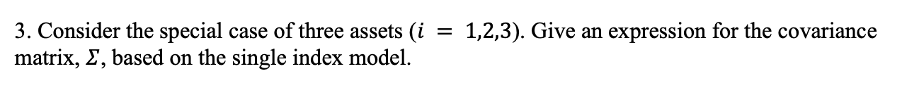
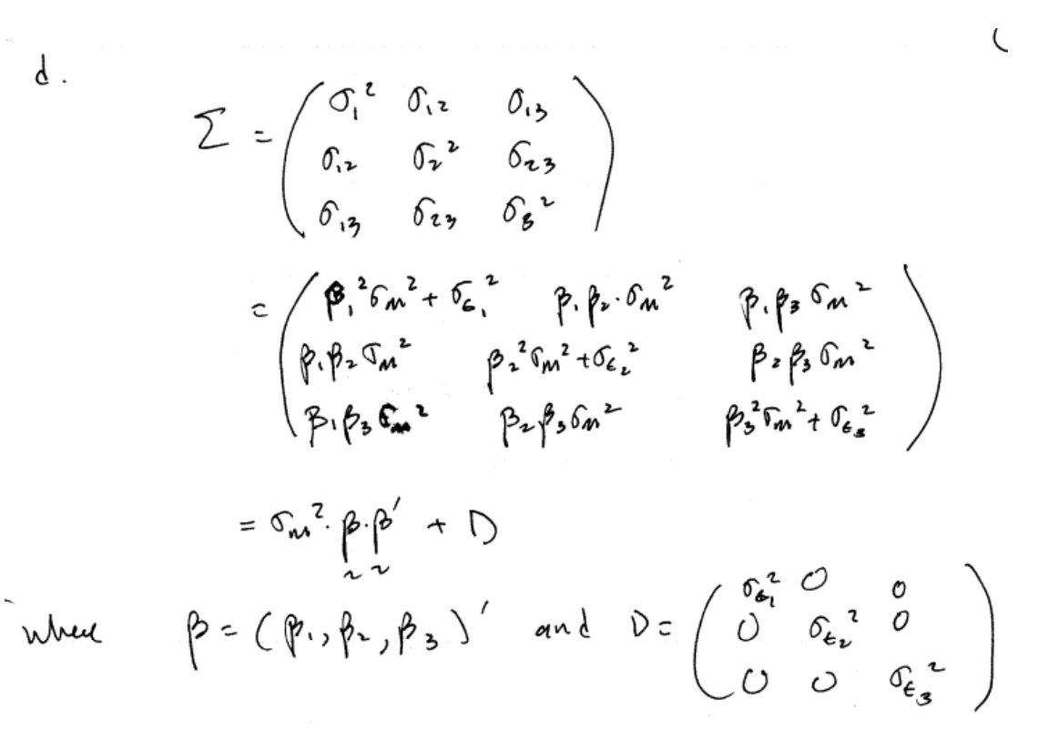
It is useful to examine the SI covariance matrix (16.19) for a three asset portfolio. In this case, we have \[\begin{align*} R_{it} & =\alpha_{i}+\beta_{i}R_{Mt}+\varepsilon_{it},\text{ }i=1,2,3\\ \sigma_{i}^{2} & =\mathrm{var}(R_{it})=\beta_{i}^{2}\sigma_{M}^{2}+\sigma_{\varepsilon,i}^{2}\\ \sigma_{ij} & =\mathrm{cov}(R_{it},R_{jt})=\sigma_{M}^{2}\beta_{i}\beta_{j} \end{align*}\] The \(3\times3\) covariance matrix is \[\begin{align*} \Sigma & =\left(\begin{array}{ccc} \sigma_{1}^{2} & \sigma_{12} & \sigma_{13}\\ \sigma_{12} & \sigma_{2}^{2} & \sigma_{23}\\ \sigma_{13} & \sigma_{23} & \sigma_{3}^{2} \end{array}\right)\\ & =\left(\begin{array}{ccc} \beta_{1}^{2}\sigma_{M}^{2}+\sigma_{\varepsilon,1}^{2} & \sigma_{M}^{2}\beta_{1}\beta_{2} & \sigma_{M}^{2}\beta_{1}\beta_{3}\\ \sigma_{M}^{2}\beta_{1}\beta_{2} & \beta_{2}^{2}\sigma_{M}^{2}+\sigma_{\varepsilon,2}^{2} & \sigma_{M}^{2}\beta_{2}\beta_{3}\\ \sigma_{M}^{2}\beta_{1}\beta_{3} & \sigma_{M}^{2}\beta_{2}\beta_{3} & \beta_{3}^{2}\sigma_{M}^{2}+\sigma_{\varepsilon,3}^{2} \end{array}\right)\\ & =\sigma_{M}^{2}\left(\begin{array}{ccc} \beta_{1}^{2} & \beta_{1}\beta_{2} & \beta_{1}\beta_{3}\\ \beta_{1}\beta_{2} & \beta_{2}^{2} & \beta_{2}\beta_{3}\\ \beta_{1}\beta_{3} & \beta_{2}\beta_{3} & \beta_{3}^{2} \end{array}\right)+\left(\begin{array}{ccc} \sigma_{\varepsilon,1}^{2} & 0 & 0\\ 0 & \sigma_{\varepsilon,2}^{2} & 0\\ 0 & 0 & \sigma_{\varepsilon,3}^{2} \end{array}\right). \end{align*}\] The first matrix shows the return variance and covariance contributions due to the market returns, and the second matrix shows the contributions due to the asset specific errors. Define \(\beta =(\beta_{1},\beta_{2},\beta_{3})^{\prime}.\) Then \[\begin{eqnarray*} \sigma_{M}^{2}\beta \beta ^{\prime} & = & \sigma_{M}^{2}\left(\begin{array}{c} \beta_{1}\\ \beta_{2}\\ \beta_{3} \end{array}\right)\left(\begin{array}{ccc} \beta_{1} & \beta_{2} & \beta_{3}\end{array}\right)=\sigma_{M}^{2}\left(\begin{array}{ccc} \beta_{1}^{2} & \beta_{1}\beta_{2} & \beta_{1}\beta_{3}\\ \beta_{1}\beta_{2} & \beta_{2}^{2} & \beta_{2}\beta_{3}\\ \beta_{1}\beta_{3} & \beta_{2}\beta_{3} & \beta_{3}^{2} \end{array}\right),\\ \mathbf{D} & = & \mathrm{diag}(\sigma_{\varepsilon,1}^{2},\sigma_{\varepsilon,2}^{2},\sigma_{\varepsilon,3}^{2})=\left(\begin{array}{ccc} \sigma_{\varepsilon,1}^{2} & 0 & 0\\ 0 & \sigma_{\varepsilon,2}^{2} & 0\\ 0 & 0 & \sigma_{\varepsilon,3}^{2} \end{array}\right), \end{eqnarray*}\] and so \[ \Sigma=\sigma_{M}^{2}\beta \beta ^{\prime}+\mathbf{D}. \]
The matrix form of the SI model (16.18) - (16.20) is useful for portfolio analysis. For example, consider a portfolio with \(N\times1\) weight vector \(\mathbf{x}=(x_{1},\ldots,x_{N})^{\prime}.\) Using (16.17), the SI model for the portfolio return \(R_{p,t}=\mathbf{x}^{\prime}R_{t}\) is \[\begin{eqnarray*} R_{p,t} & = & \mathbf{x}^{\prime}(\alpha+\beta R_{Mt}+\epsilon_{t})\\ & = & \mathbf{x}^{\prime}\alpha+\mathbf{x}^{\prime}\beta R_{Mt}+\mathbf{x}^{\prime}\epsilon_{t}\\ & = & \alpha_{p}+\beta_{p}R_{Mt}+\epsilon_{p,t}, \end{eqnarray*}\] where \(\alpha_{p}=\mathbf{x}^{\prime}\alpha\), \(\beta_{p}=\mathbf{x}^{\prime}\beta\) and \(\epsilon_{p,t}=\mathbf{x}^{\prime}\epsilon_{t}\).
16.3 Monte Carlo Simulation of the SI Model
To give a first step reality check for the SI model, consider simulating data from the SI model for a single asset. The steps to create a Monte Carlo simulation from the SI model are:
- Fix values for the SI model parameters \(\alpha\), \(\beta\), \(\sigma_{\epsilon}\), \(\mu_{M}\) and \(\sigma_{M}\)
- Determine the number of simulated returns, \(T\), to create.
- Use a computer random number generator to simulate \(T\) iid values of \(R_{Mt}\sim N(\mu_{M},\sigma_{M}^{2})\) and \(\epsilon_{t}\sim N(0,\sigma_{\epsilon}^{2})\), where \(R_{Mt}\) is simulated independently from \(\epsilon_{t}\).
- Create the simulated asset returns \(\tilde{R}_{t}=\alpha+\beta\tilde{R}_{M}\)+\(\tilde{\epsilon}_{t}\) for \(t=1,\ldots,T\)
The following example illustrates simulating SI model returns for Boeing.
Consider simulating monthly returns on Boeing from the SI model where the S&P 500 index is used as the market index. The SI model parameters are calibrated from the actual monthly returns on Boeing and the S&P 500 index using sample statistics, as discussed in the next section, and are given by: \[ \alpha_{BA}=0.005,\,\beta_{BA}=0.98,\,\sigma_{\epsilon,BA}=0.08,\,\mu_{M}=0.003,\,\sigma_{M}=0.048. \] These values are set in R using:
The simulated returns for the S&P 500 index and Boeing are created using:
n.sim = nrow(siRetS)
set.seed(123)
sp500.sim = rnorm(n.sim, mu.sp500, sd.sp500)
e.BA.sim = rnorm(n.sim, 0, sd.e.BA)
BA.sim = alpha.BA + beta.BA*sp500.sim + e.BA.sim
BA.sim = xts(BA.sim, index(siRetS))
sp500.sim = xts(sp500.sim, index(siRetS))
colnames(BA.sim) = "BA.sim"
colnames(sp500.sim) = "SP500.sim"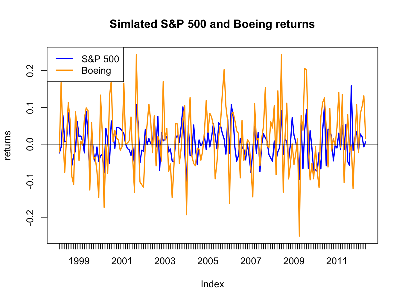
Figure 16.5: Simulated SI model monthly returns on the S&P 500 index and Boeing.
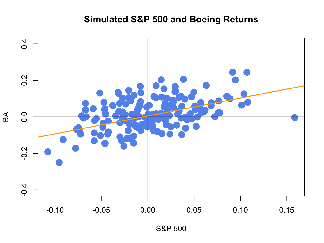
Figure 16.6: Simulated SI model monthly returns on the S&P 500 index and Boeing. The orange line is the equation \(R_{BA,t}=\alpha_{BA}+\beta_{BA}R_{Mt}=0.005+0.98\times R_{Mt}.\)
The simulate returns are illustrated in Figures 16.5 and 16.6. The time plot and scatterplot of the simulated returns on the S&P 500 index look much like the corresponding plots of the actual returns shows in the top left panels of Figures 16.2 and 16.4, respectively. Hence, the SI model for the S&P 500 index and Boeing passes the first step reality check. In Figure 16.6, the line \(\alpha_{i}+\beta_{i}R_{Mt}=0.005+0.98R_{Mt}\) is shown in orange. This line represents the predictions of Boeing’s return given the S&P 500 return. For example, if \(R_{Mt}=0.05\) then the predicted return for Boeing is \(R_{BA}=0.005+0.98\times(0.05)=0.054\). The differences between the observed Boeing returns and (blue dots) and the predicted returns (orange line) are the asset specific error terms. These are the random asset specific news components. The standard deviation of these components, \(\sigma_{\epsilon,BA}=0.08\), represents the typical magnitude of these components. Here, we would not be too surprised if the observed Boeing return is \(0.08\) above or below the orange line. How close the Boeing returns are to the predicted returns is determined by the \(R^{2}\) value given by (16.15). Here, \(\sigma_{BA}^{2}=\beta_{BA}^{2}\sigma_{M}^{2}+\sigma_{\epsilon,BA}^{2}=(0.98)^{2}(0.048)^{2}+(0.08)^{2}=0.00861\) and so \(R^{2}=(0.98)^{2}(0.048)^{2}/0.00861=0.257\). Hence, 25.7% of the variability (risk) of Boeing returns are explained by the variability of the S&P 500 returns. As a result, 74.3% \((1-R^{2}=0.743)\) of the variability of Boeing returns are due to the random asset specific terms.
\(\blacksquare\)
16.4 Estimation of SI Model
Consider the SI model (16.1) - (16.5). The asset specific parameters to be estimated are \(\alpha_{i}\), \(\beta_{i}\) and \(\sigma_{\epsilon,i}^{2}\), \((i=1,\ldots,N)\), and the market parameters to be estimated are \(\mu_{M}\) and \(\sigma_{M}^{2}\). These parameters can be estimated using the plug-in principle, linear regression, and maximum likelihood. All methods give essentially the same estimators for the SI model parameters.
16.4.1 Plug-in principle estimates
Let \(\{(r_{it},r_{Mt})\}_{t=1}^{T}\) denote a sample of size \(T\) of observed returns on asset \(i\) and the market return which are assumed to be generated from the SI model. (16.1) - (16.12). Recall, the plug-in principle says to estimate population model parameters using appropriate sample statistics. For the market parameters, the plug-in principle estimates are the same as the CER model estimates \[\begin{eqnarray*} \hat{\mu}_{M} & = & \frac{1}{T}\sum_{t=1}^{T}r_{Mt},\\ \hat{\sigma}_{M}^{2} & = & \frac{1}{T-1}\sum_{t=1}^{T}(r_{Mt}-\hat{\mu}_{M})^{2}. \end{eqnarray*}\] From (16.13) - (16.6) we see that \(\alpha_{i}\) and \(\beta_{i}\) are functions of population parameters \[\begin{eqnarray*} \alpha_{i} & = & \mu_{i}-\beta_{i}\mu_{M},\\ \beta_{i} & = & \frac{\mathrm{cov}(R_{it},R_{Mt})}{\mathrm{var}(R_{Mt})}=\frac{\sigma_{iM}}{\sigma_{M}^{2}}. \end{eqnarray*}\] The corresponding plug-in principle estimates are then: \[\begin{eqnarray} \hat{\alpha}_{i} & = & \hat{\mu}_{i}-\hat{\beta}_{i}\hat{\mu}_{M},\tag{16.21}\\ \hat{\beta}_{i} & = & \frac{\hat{\sigma}_{iM}}{\hat{\sigma}_{M}^{2}},\tag{16.22} \end{eqnarray}\] where \[\begin{eqnarray*} \hat{\mu}_{i} & = & \frac{1}{T}\sum_{t=1}^{T}r_{it},\\ \hat{\sigma}_{iM} & = & \frac{1}{T-1}\sum_{t=1}^{T}(r_{it}-\hat{\mu}_{i})(r_{Mt}-\hat{\mu}_{M}). \end{eqnarray*}\]
Given the plug-in principle estimates \(\hat{\alpha}_{i}\) and \(\hat{\beta}_{i}\), the plug-in principle estimate of \(\epsilon_{it}\) is \[\begin{equation} \hat{\varepsilon}_{it}=r_{it}-\hat{\alpha}_{i}-\hat{\beta}_{i}r_{Mt},\,t=1,\ldots,T.\tag{16.23} \end{equation}\] Using (16.23), the plug-in principle estimate of \(\sigma_{\epsilon,i}^{2}\) is the sample variance of \(\{\hat{\epsilon}_{it}\}_{t=1}^{T}\) (adjusted for the number of degrees of freedom): \[\begin{align} \hat{\sigma}_{\varepsilon,i}^{2} & =\frac{1}{T-2}\sum_{t=1}^{T}\hat{\varepsilon}_{t}^{2}=\frac{1}{T-2}\sum_{t=1}^{T}\left(r_{it}-\hat{\alpha}_{i}-\hat{\beta}_{i}r_{Mt}\right)^{2}.\tag{16.24} \end{align}\]
Plug-in principle estimates of \(R^{2}\) based on (16.15) can be computed using \[\begin{align} \hat{R}^{2} & =\frac{\hat{\beta}_{i}^{2}\hat{\sigma}_{M}^{2}}{\hat{\sigma}_{i}^{2}}=1-\frac{\hat{\sigma}_{\varepsilon,i}^{2}}{\hat{\sigma}_{i}^{2}}.\tag{16.25} \end{align}\]
Consider computing the plug-in principle estimates for \(\alpha_{i},\) \(\beta_{i}\) and \(\sigma_{\epsilon,i}^{2}\) from the example data using the formulas (16.21), (16.22) and (16.24), respectively. First, extract the sample statistics \(\hat{\mu}_{i}\), \(\hat{\sigma}_{iM}\), \(\hat{\mu}_{M}\), and \(\hat{\sigma}_{M}^{2}\):
assetNames = colnames(siRetS)[1:4]
muhat = colMeans(siRetS)
sig2hat = diag(covmatHat)
covAssetsSp500 = covmatHat[assetNames, "SP500"]
Next, estimate \(\hat{\beta}_{i}\) using
##    BA   JWN  MSFT  SBUX
## 0.978 1.485 1.303 1.057
Here, we see that \(\hat{\beta}_{BA}\) and \(\hat{\beta}_{SBUX}\) are very close to one and that \(\hat{\beta}_{JWN}\) and \(\hat{\beta}_{MSFT}\) are slightly bigger than one. Using the estimates of \(\hat{\beta}_{i}\) and the sample statistics \(\hat{\mu}_{i}\) and \(\hat{\mu}_{M}\) the estimates for \(\hat{\alpha}_{i}\) are
##      BA     JWN    MSFT    SBUX
## 0.00516 0.01231 0.00544 0.01785
All of the estimates of \(\hat{\alpha}_{i}\) are close to zero. The estimates of \(\sigma_{\epsilon,i}^{2}\) can be computed using:
sig2eHat = rep(0, length(assetNames))
names(sig2eHat) = assetNames
for (aName in assetNames) {
     eHat = siRetS[, aName] - alphaHat[aName] - betaHat[aName]*siRetS[, "SP500"]
     sig2eHat[aName] = crossprod(eHat)/(length(eHat) - 2)
}
sig2eHat
## BA JWN MSFT SBUX
## 0.00581 0.00994 0.00646 0.00941Lastly, the estimates of \(R^{2}\) can be computed using
##    BA   JWN  MSFT  SBUX
## 0.270 0.334 0.373 0.210
\(\blacksquare\)
16.4.2 Least squares estimates
The SI model representation (16.1) shows that returns are a linear function of the market return and an asset specific error term \[ R_{it}=\alpha_{i}+\beta_{i}R_{Mt}+\epsilon_{it}, \] here \(\alpha_{i}\) is the intercept and \(\beta_{i}\) is the slope. Least squares regression is a method for estimating \(\alpha_{i}\) and \(\beta_{i}\) by finding the “best fitting” line to the scatterplot of returns where \(R_{it}\) is on the vertical axis and \(R_{Mt}\) is on the horizontal axis.
{[}Insert Figure here{]} To be completed…
To see how the method of least squares determines the “best fitting” line, consider the scatterplot of the sample returns on Boeing and the S&P 500 index illustrated in Figure xxx. In the figure, the black line is a fitted line with initial guess \(\hat{\alpha}_{BA}=0\) and \(\hat{\beta}_{BA}=0.5.\) The differences between the observed returns (blue dots) and the values on the fitted line are the estimated errors \(\hat{\epsilon}_{BA,t}=r_{BA,t}-\hat{\alpha}_{BA}-\hat{\beta}_{BA}r_{Mt}=r_{BA,t}-0-0.5\times R_{Mt}.\) Some estimated errors are big and some are small. The overall fit of the line can be measured using a statistic based on all \(t=1,\ldots,T\) of the estimated errors. A natural choice is the sum of the errors \(\sum_{t=1}^{T}\hat{\epsilon}_{t}\). However, this choice can be misleading due to the canceling out of large positive and negative errors. To avoid this problem, it is better to measure the overall fit using \(\sum_{t=1}^{T}\hat{|\epsilon}_{t}|\) or \(\sum_{t=1}^{T}\hat{\epsilon}_{t}^{2}.\) Then the best fitting line can be determined by finding the intercept and slope values that minimize \(\sum_{t=1}^{T}\hat{|\epsilon}_{t}|\) or \(\sum_{t=1}^{T}\hat{\epsilon}_{t}^{2}.\)
The method of least squares regression defines the “best fitting” line by finding the intercept and slope values that minimize the sum of squared errors \[\begin{equation} \mathrm{SSE}(\hat{\alpha}_{i},\hat{\beta}_{i})=\sum_{t=1}^{T}\hat{\epsilon}_{it}^{2}=\sum_{t=1}^{T}\left(r_{it}-\hat{\alpha}_{i}-\hat{\beta}_{i}r_{Mt}\right)^{2}.\tag{16.26} \end{equation}\] Because \(\mathrm{SSE}(\hat{\alpha},\hat{\beta})\) is a continuous and differential function of \(\hat{\alpha}_{i}\) and \(\hat{\beta}_{i}\), the minimizing values of \(\hat{\alpha}_{i}\) and \(\hat{\beta}_{i}\) can be determined using simple calculus. The first order conditions for a minimum are: \[\begin{align} 0 & =\frac{\partial\mathrm{SSE}(\hat{\alpha}_{i},\hat{\beta}_{i})}{\partial\hat{\alpha}_{i}}=-2\sum_{t=1}^{T}(r_{it}-\hat{\alpha}_{i}-\hat{\beta}_{i}r_{Mt})=-2\sum_{t=1}^{T}\hat{\varepsilon}_{it},\tag{16.27}\\ 0 & =\frac{\partial\mathrm{SSE}(\hat{\alpha}_{i},\hat{\beta}_{i})}{\partial\hat{\beta}_{i}}=-2\sum_{t=1}^{T}(r_{it}-\hat{\alpha}_{i}-\hat{\beta}_{i}r_{Mt})r_{Mt}=-2\sum_{t=1}^{T}\hat{\varepsilon}_{it}r_{Mt}.\tag{16.28} \end{align}\] These are two linear equations in two unknowns which can be re-expressed as \[\begin{eqnarray*} \hat{\alpha}_{i}T+\hat{\beta}_{i}\sum_{t=1}^{T}r_{Mt} & = & \sum_{t=1}^{T}r_{it},\\ \hat{\alpha}_{i}\sum_{t=1}^{T}r_{Mt}+\hat{\beta}_{i}\sum_{t=1}^{T}r_{Mt}^{2} & = & \sum_{t=1}^{T}r_{it}r_{Mt}. \end{eqnarray*}\] Using matrix algebra, we can write these equations as: \[\begin{equation} \left(\begin{array}{cc} T & \sum_{t=1}^{T}r_{Mt}\\ \sum_{t=1}^{T}r_{Mt} & \sum_{t=1}^{T}r_{Mt}^{2} \end{array}\right)\left(\begin{array}{c} \hat{\alpha}_{i}\\ \hat{\beta}_{i} \end{array}\right)=\left(\begin{array}{c} \sum_{t=1}^{T}r_{it}\\ \sum_{t=1}^{T}r_{it}r_{Mt} \end{array}\right),\tag{16.29} \end{equation}\] which is of the form \(\mathbf{Ax}=\mathbf{b}\) with \[ \mathbf{A}=\left(\begin{array}{cc} T & \sum_{t=1}^{T}r_{Mt}\\ \sum_{t=1}^{T}r_{Mt} & \sum_{t=1}^{T}r_{Mt}^{2} \end{array}\right),\,\mathbf{x}=\left(\begin{array}{c} \hat{\alpha}_{i}\\ \hat{\beta}_{i} \end{array}\right),\,\mathbf{b}=\left(\begin{array}{c} \sum_{t=1}^{T}r_{it}\\ \sum_{t=1}^{T}r_{it}r_{Mt} \end{array}\right). \] Hence, we can determine \(\hat{\alpha}_{i}\) and \(\hat{\beta}_{i}\) by solving \(\mathbf{x}=\mathbf{A}^{-1}\mathbf{b}.\) Now,98 \[\begin{eqnarray*} \mathbf{A}^{-1} & = & \frac{1}{\mathrm{det}(\mathbf{A})}\left(\begin{array}{cc} \sum_{t=1}^{T}r_{Mt}^{2} & -\sum_{t=1}^{T}r_{Mt}\\ -\sum_{t=1}^{T}r_{Mt} & T \end{array}\right),\\ \mathrm{det}(\mathbf{A}) & = & T\sum_{t=1}^{T}r_{Mt}^{2}-\left(\sum_{t=1}^{T}r_{Mt}\right)^{2}=T\sum_{t=1}^{T}\left(r_{Mt}-\hat{\mu}_{M}\right)^{2},\\ \hat{\mu}_{M} & = & \frac{1}{T}\sum_{t=1}^{T}r_{Mt}. \end{eqnarray*}\] Consequently, \[\begin{equation} \left(\begin{array}{c} \hat{\alpha}_{i}\\ \hat{\beta}_{i} \end{array}\right)=\frac{1}{T\sum_{t=1}^{T}\left(r_{Mt}-\hat{\mu}_{M}\right)^{2}}\left(\begin{array}{cc} \sum_{t=1}^{T}r_{Mt}^{2} & -\sum_{t=1}^{T}r_{Mt}\\ -\sum_{t=1}^{T}r_{Mt} & T \end{array}\right)\left(\begin{array}{c} \sum_{t=1}^{T}r_{it}\\ \sum_{t=1}^{T}r_{it}r_{Mt} \end{array}\right)\tag{16.30} \end{equation}\] and so \[\begin{eqnarray} \hat{\alpha}_{i} & = & \frac{\sum_{t=1}^{T}r_{Mt}^{2}\sum_{t=1}^{T}r_{it}-\sum_{t=1}^{T}r_{Mt}^{2}\sum_{t=1}^{T}r_{it}r_{Mt}}{T\sum_{t=1}^{T}\left(r_{Mt}-\hat{\mu}_{M}\right)^{2}},\tag{16.31}\\ \hat{\beta}_{i} & = & \frac{T\sum_{t=1}^{T}r_{it}r_{Mt}-\sum_{t=1}^{T}r_{Mt}\sum_{t=1}^{T}r_{it}}{T\sum_{t=1}^{T}\left(r_{Mt}-\hat{\mu}_{M}\right)^{2}}.\tag{16.32} \end{eqnarray}\] After a little bit of algebra (see end-of-chapter exercises) it can be shown that \[\begin{eqnarray*} \hat{\alpha}_{i} & = & \hat{\mu}_{i}-\hat{\beta}_{i}\hat{\mu}_{M},\\ \hat{\beta}_{i} & = & \frac{\hat{\sigma}_{iM}}{\hat{\sigma}_{M}^{2}}, \end{eqnarray*}\] which are plug-in estimates for \(\hat{\alpha}_{i}\) and \(\hat{\beta}_{i}\) determined earlier. Hence, the least squares estimates of \(\hat{\alpha}_{i}\) and \(\hat{\beta}_{i}\) are identical to the plug-in estimates.
The solution for the least squares estimates in (16.30) has an elegant representation using matrix algebra. To see this, define the \(T\times1\) vectors \(\mathbf{r}_{i}=(r_{i1},\ldots,r_{iT})^{\prime}\), \(\mathbf{r}_{M}=(r_{M1},\ldots,r_{MT})^{\prime}\) and \(\mathbf{1}=(1,\ldots,1)^{\prime}\). Then we can re-write (16.29) as \[ \left(\begin{array}{cc} \mathbf{1}^{\prime}\mathbf{1} & \mathbf{1}^{\prime}\mathbf{r}_{M}\\ \mathbf{1}^{\prime}\mathbf{r}_{M} & \mathbf{r}_{M}^{\prime}\mathbf{r}_{M} \end{array}\right)\left(\begin{array}{c} \hat{\alpha}_{i}\\ \hat{\beta}_{i} \end{array}\right)=\left(\begin{array}{c} \mathbf{1}^{\prime}\mathbf{r}_{i}\\ \mathbf{r}_{M}^{\prime}\mathbf{r}_{i} \end{array}\right) \] or \[\begin{equation} \mathbf{X}^{\prime}\mathbf{X}\hat{\gamma}_{i}=\mathbf{X}^{\prime}\mathbf{r}_{i}\tag{16.33} \end{equation}\] where \(\mathbf{X}=(\begin{array}{cc} \mathbf{1} & \mathbf{r}_{M})\end{array}\)is a \(T\times2\) matrix and \(\hat{\gamma}=(\hat{\alpha}_{i},\hat{\beta}_{i})^{\prime}\). Provided \(\mathbf{X}^{\prime}\mathbf{X}\) is invertible, solving (16.33) for \(\hat{\gamma}_{i}\) gives the least squares estimates in matrix form: \[\begin{equation} \hat{\gamma}_{i}=\left(\mathbf{X}^{\prime}\mathbf{X}\right)^{-1}\mathbf{X}^{\prime}\mathbf{r}_{i}.\tag{16.34} \end{equation}\] The matrix form solution (16.34) is especially convenient for computation in R.
The least squares estimates of \(\epsilon_{t}\), \(\sigma_{\epsilon,i}^{2}\) and \(R^{2}\) are the same as the plug-in estimators (16.23), (16.24) and (16.25), respectively. In the context of least squares estimation, the estimate \(\hat{\sigma}_{\epsilon,i}=\sqrt{\hat{\sigma}_{\epsilon,i}^{2}}\) is called the standard error of the regression and measures the typical magnitude of \(\hat{\epsilon}_{t}\) (difference between observed return and fitted regression line).
16.4.3 Simple linear regression in R
- don’t do regression examples until statistical theory is discussed
- computing least squares estimates using matrix algebra formulas
- computing least squares estimates using
lm()- See discussion from my regression chapter in MFTSR
- describe structure of
lm()function, extractor and method functions
- Do analysis of example data To be completed…
16.4.4 Maximum likelihood estimates
The SI model parameters can also be estimated using the method of maximum likelihood, which was introduced in chapter (GARCH estimation chapter). To construct the likelihood function, we use property () of the SI model that conditional on \(R_{Mt}=r_{Mt}\) the distribution of \(R_{it}\) is normal with mean \(\alpha_{i}+\beta_{i}r_{Mt}\) and variance \(\sigma_{\epsilon,i}^{2}\). The pdf of \(R_{it}|R_{Mt}=r_{mt}\) is then \[ f(r_{it}|r_{mt},\theta_{i})=(2\pi\sigma_{\varepsilon,i}^{2})^{-1/2}\exp\left(\frac{-1}{2\sigma_{\varepsilon,i}^{2}}\left(r_{it}-\alpha_{i}+\beta_{i}r_{Mt}\right)^{2}\right),\,t=1,\ldots,T, \] where \(\theta_{i}=(\alpha_{i},\beta_{i},\sigma_{\epsilon,i}^{2})^{\prime}\). Given a sample \(\{(r_{it},r_{Mt})\}_{t=1}^{T}=\{\mathbf{r}_{i},\mathbf{r}_{M}\}\) of observed returns on asset \(i\) and the market return, which are assumed to be generated from the SI model, the joint density of asset returns given the market returns is \[\begin{eqnarray*} f(\mathbf{r}_{i}|\mathbf{r}_{m}) & = & \prod_{t=1}^{T}(2\pi\sigma_{\varepsilon,i}^{2})^{-1/2}\exp\left(\frac{-1}{2\sigma_{\varepsilon,i}^{2}}\left(r_{it}-\alpha_{i}+\beta_{i}r_{Mt}\right)^{2}\right)\\ & = & (2\pi\sigma_{\varepsilon,i}^{2})^{-T/2}\exp\left(\frac{-1}{2\sigma_{\varepsilon,i}^{2}}\sum_{t=1}^{T}\left(r_{it}-\alpha_{i}+\beta_{i}r_{Mt}\right)^{2}\right)\\ & = & (2\pi\sigma_{\varepsilon,i}^{2})^{-T/2}\exp\left(\frac{-1}{2\sigma_{\varepsilon,i}^{2}}\mathrm{SSE}(\alpha_{i},\beta_{i})\right). \end{eqnarray*}\] where \(\mathrm{SSE}(\alpha_{i},\beta_{i})\) is the sum of squared residuals (16.26) used to determine the least squares estimates. The log-likelihood function for \(\theta_{i}\) is then \[\begin{eqnarray} lnL(\theta_{i}|\mathbf{r}_{i},\mathbf{r}_{M}) & = & \frac{-T}{2}\ln(2\pi)-\frac{T}{2}\ln(\sigma_{\varepsilon,i}^{2})-\frac{1}{2\sigma_{\varepsilon,i}^{2}}\mathrm{SSE}(\alpha_{i},\beta_{i}).\tag{16.35} \end{eqnarray}\] From (16.35), it can be seen that the values of \(\alpha_{i}\) and \(\beta_{i}\) that maximize the log-likelihood are the values that minimize \(\mathrm{SSE}(\alpha_{i},\beta_{i})\). Hence, the ML estimates of \(\alpha_{i}\) and \(\beta_{i}\) are the least squares estimates.
To find the ML estimate for \(\sigma_{\epsilon,i}^{2}\), plug the ML estimates of \(\alpha_{i}\) and \(\beta_{i}\) into (16.35) giving \[ lnL(\hat{\alpha}_{i},\hat{\beta}_{i},\sigma_{\epsilon,i}^{2}|\mathbf{r}_{i},\mathbf{r}_{M})=\frac{-T}{2}\ln(2\pi)-\frac{T}{2}\ln(\sigma_{\varepsilon,i}^{2})-\frac{1}{2\sigma_{\varepsilon,i}^{2}}\mathrm{SSE}(\hat{\alpha}_{i},\hat{\beta}_{i}). \] Maximization with respect to \(\sigma_{\epsilon,i}^{2}\) gives the first order condition \[ \frac{\partial lnL(\hat{\alpha}_{i},\hat{\beta}_{i},\sigma_{\epsilon,i}^{2}|\mathbf{r}_{i},\mathbf{r}_{M})}{\partial\sigma_{\epsilon,i}^{2}}=-\frac{T}{2\hat{\sigma}_{\epsilon,i}^{2}}+\frac{1}{2\left(\hat{\sigma}_{\epsilon,i}^{2}\right)^{2}}\mathrm{SSE}(\hat{\alpha}_{i},\hat{\beta}_{i})=0. \] Solving for \(\hat{\sigma}_{\epsilon,i}^{2}\) gives the ML estimate for \(\sigma_{\epsilon,i}^{2}\): \[ \hat{\sigma}_{\epsilon,i}^{2}=\frac{\mathrm{SSE}(\hat{\alpha}_{i},\hat{\beta}_{i})}{T}=\frac{1}{T}\sum_{t=1}^{T}\hat{\epsilon}_{t}^{2}, \] which is plug-in principle estimate (16.24) not adjusted for degrees-of-freedom.
16.5 Statistical Properties of SI Model Estimates
To determine the statistical properties of the plug-in principle/least squares/ML estimators \(\hat{\alpha}_{i}\), \(\hat{\beta}_{i}\) and \(\hat{\sigma}_{\epsilon,i}^{2}\) in the SI model, we treat them as functions of the random variables \(\{(R_{i,t},R_{Mt})\}_{t=1}^{T}\) where \(R_{t}\) and \(R_{Mt}\) are assumed to be generated by the SI model (16.1) - (16.5).
16.5.1 Bias
In the SI model, the estimators \(\hat{\alpha}_{i}\), \(\hat{\beta}_{i}\) and \(\hat{\sigma}_{\epsilon,i}^{2}\) (with degrees-of-freedom adjustment) are unbiased: \[\begin{eqnarray*} E[\hat{\alpha}_{i}] & = & \alpha_{i},\\ E[\hat{\beta}_{i}] & = & \beta_{i},\\ E[\hat{\sigma}_{\epsilon,i}^{2}] & = & \sigma_{\epsilon,i}^{2}. \end{eqnarray*}\] To shows that \(\hat{\alpha}_{i}\) and \(\hat{\beta}_{i}\) are unbiased, it is useful to consider the SI model for asset \(i\) in matrix form for \(t=1,\ldots,T\): \[ \mathbf{R}_{i}=\alpha_{i}\mathbf{1}+\beta_{i}\mathbf{R}_{M}+\epsilon_{i}=\mathbf{X}\gamma_{i}+\epsilon_{i}, \] where \(\mathbf{R}_{i}=(R_{i1},\ldots,R_{iT})^{\prime},\) \(\mathbf{R}_{M}=(R_{M1},\ldots,R_{MT})^{\prime}\), \(\epsilon_{i}=(\epsilon_{i1},\ldots,\epsilon_{iT})^{\prime}\), \(\mathbf{1}=(1,\ldots,1)^{\prime}\), \(\mathbf{X}=(\begin{array}{cc} \mathbf{1} & \mathbf{R}_{M})\end{array},\) and \(\gamma_{i}=(\alpha_{i},\beta_{i})^{\prime}.\) The estimator for \(\gamma_{i}\) is \[\begin{eqnarray*} \hat{\gamma}_{i} & = & (\mathbf{X}^{\prime}\mathbf{X})^{-1}\mathbf{X}^{\prime}\mathbf{R}_{i}. \end{eqnarray*}\] Pluging in \(\mathbf{R}_{i}=\mathbf{X}\gamma_{i}+\epsilon_{i}\) gives \[\begin{eqnarray*} \hat{\gamma}_{i} & = & (\mathbf{X}^{\prime}\mathbf{X})^{-1}\mathbf{X}^{\prime}\left(\mathbf{X}\gamma_{i}+\epsilon_{i}\right)=(\mathbf{X}^{\prime}\mathbf{X})^{-1}\mathbf{X}^{\prime}\mathbf{X}\gamma_{i}+(\mathbf{X}^{\prime}\mathbf{X})^{-1}\mathbf{X}^{\prime}\epsilon_{i}\\ & = & \gamma_{i}+(\mathbf{X}^{\prime}\mathbf{X})^{-1}\mathbf{X}^{\prime}\epsilon_{i}. \end{eqnarray*}\] Then \[\begin{eqnarray*} E[\hat{\gamma}_{i}] & = & \gamma_{i}+E\left[(\mathbf{X}^{\prime}\mathbf{X})^{-1}\mathbf{X}^{\prime}\epsilon_{i}\right]\\ & = & \gamma_{i}+E\left[(\mathbf{X}^{\prime}\mathbf{X})^{-1}\mathbf{X}^{\prime}\right]E[\epsilon_{i}]\,(\mathrm{because}\,\epsilon_{it}\,\mathrm{is}\,\mathrm{independent}\,\mathrm{of}\,R_{Mt})\\ & = & \gamma_{i}\,(\mathrm{because}\,E[\epsilon_{i}]=\mathbf{0}). \end{eqnarray*}\] The derivation of \(E[\hat{\sigma}_{\epsilon,i}^{2}]=\sigma_{\epsilon,i}^{2}\) is beyond the scope of this book and can be found in graduate econometrics textbooks such as Hayashi (1980).
16.5.2 Precision
Under the assumptions of the SI model, analytic formulas for estimates of the standard errors for \(\hat{\alpha}_{i}\) and \(\hat{\beta}_{i}\) are given by: \[\begin{align} \widehat{\mathrm{se}}(\hat{\alpha}_{i}) & \approx\frac{\hat{\sigma}_{\varepsilon,i}}{\sqrt{T\cdot\hat{\sigma}_{M}^{2}}}\cdot\sqrt{\frac{1}{T}\sum_{t=1}^{T}r_{Mt}^{2}},\tag{16.36}\\ \widehat{\mathrm{se}}(\hat{\beta}_{i}) & \approx\frac{\hat{\sigma}_{\varepsilon,i}}{\sqrt{T\cdot\hat{\sigma}_{M}^{2}}},\tag{16.37} \end{align}\] where “\(\approx\)” denotes an approximation based on the CLT that gets more accurate the larger the sample size. Remarks:
- \(\widehat{\mathrm{se}}(\hat{\alpha}_{i})\) and \(\widehat{\mathrm{se}}(\hat{\beta}_{i})\) are smaller the smaller is \(\hat{\sigma}_{\varepsilon,i}\). That is, the closer are returns to the fitted regression line the smaller are the estimation errors in \(\hat{\alpha}_{i}\) and \(\hat{\beta}_{i}\).
- \(\widehat{\mathrm{se}}(\hat{\beta}_{i})\) is smaller the larger is \(\hat{\sigma}_{M}^{2}\). That is, the greater the variability in the market return \(R_{Mt}\) the smaller is the estimation error in the estimated slope coefficient \(\hat{\beta}_{i}\). This is illustrated in Figure xxx. The left panel shows a data sample from the SI model with a small value of \(\hat{\sigma}_{M}^{2}\) and the right panel shows a sample with a large value of \(\hat{\sigma}_{M}^{2}\). The right panel shows that the high variability in \(R_{Mt}\) makes it easier to identify the slope of the line.
- Both \(\widehat{\mathrm{se}}(\hat{\alpha}_{i})\) and \(\widehat{\mathrm{se}}(\hat{\beta}_{i})\) go to zero as the sample size, \(T\), gets large. Since \(\hat{\alpha}_{i}\) and \(\hat{\beta}_{i}\) are unbiased estimators, this implies that they are also consistent estimators. That is, they converge to the true values \(\alpha_{i}\) and \(\beta_{i}\), respectively, as \(T\rightarrow\infty\).
- In R, the standard error values (16.36) and (16.37) are computed using the
summary()function on an “lm” object.
There are no easy formulas for the estimated standard errors for \(\hat{\sigma}_{\epsilon,i}^{2}\), \(\hat{\sigma}_{\varepsilon,i}\) and \(\hat{R}^{2}\). Estimated standard errors for these estimators, however, can be easily computed using the bootstrap.
to be completed
\(\blacksquare\)
16.5.3 Sampling distribution and confidence intervals.
Using arguments based on the CLT, it can be shown that for large enough \(T\) the estimators \(\hat{\alpha}_{i}\) and \(\hat{\beta}_{i}\) are approximately normally distributed: \[\begin{eqnarray*} \hat{\alpha}_{i} & \sim & N(\alpha_{i},\widehat{\mathrm{se}}(\hat{\alpha}_{i})^{2}),\\ \hat{\beta}_{i} & \sim & N(\beta_{i},\widehat{\mathrm{se}}(\hat{\beta}_{i})^{2}), \end{eqnarray*}\] where \(\widehat{\mathrm{se}}(\hat{\alpha}_{i})\) and \(\widehat{\mathrm{se}}(\hat{\beta}_{i})\) are given by (16.36) and (16.37), respectively.
16.6 Further Reading: Single Index Model
To be completed …
16.7 Problems: Single Index Model
16.8 Solutions to Selected Problems
{Ruppert} Ruppert, D.A.. , Springer-Verlag.
{MartinSchererYollin}Martin, R.D., Scherer, B., and Yollin, G. (2016).
The single index model is also called the* market model* or the single factor model.↩︎
The S&P 500 index is a value weighted index and so is not equal to an equally weighted portfolio of the stocks in the S&P 500 index. However, since most stocks in the S&P 500 index have large market capitalizations the values weights are not too different from equal weights.↩︎
The matrix \(\mathbf{A}\) is invertible provided \(\mathrm{det}(A)\neq0.\) This requires the sample variance of \(R_{Mt}\) to be non-zero. ↩︎