2 Review of Random Variables
Updated: Februrary 3, 2022
Copyright © Eric Zivot 2022
This chapter reviews the probability concepts that are necessary for the modeling and statistical analysis of financial data presented in this book. This material is typically covered in an introductory probability and statistics course using calculus. In the course of the review, many examples related to finance will be presented and some important risk concepts, such as value-at-risk, will be introduced. The examples will also show how to use R for probability calculations and working with probability distributions.
The chapter is outlined as follows. Section 2.1 reviews univariate random variables and properties of univariate probability distributions. Important univariate distributions, such as the normal distribution, that are used throughout the book for modeling financial data, are described in detail. Section 2.2 covers bivariate probability distributions for two random variables. The concepts of dependence and independence between two random variables are discussed. The measures of linear dependence between two random variables, covariance and correlation, are defined and the bivariate normal distribution is introduced. Properties of linear combinations of two random variables are given and illustrated using an example to describe the return and risk properties of a portfolio of two assets. More than two random variables and Multivariate distributions are briefly discussed in section 2.3.
The R packages used in this chapter are mvtnorm and sn. Make sure these packages are downloaded and installed prior to replicating the R examples in this chapter.
2.1 Random Variables
We start with the basic definition of a random variable:
Definition 2.1 A random variable, \(X\), is a variable that can take on a given set of values, called the sample space and denoted \(S_{X}\), where the likelihood of the values in \(S_{X}\) is determined by \(X\)’s probability distribution function (pdf).
Consider the price of Microsoft stock next month, \(P_{t+1}\). Since \(P_{t+1}\) is not known with certainty today (\(t\)), we can consider it as a random variable. \(P_{t+1}\) must be positive, and realistically it can’t get too large. Therefore, the sample space is the set of positive real numbers bounded above by some large number: \(S_{P_{t+1}}=\{P_{t+1}:P_{t+1}\in[0,M],~M>0\}\). It is an open question as to what is the best characterization of the probability distribution of stock prices. The log-normal distribution is one possibility.9
\(\blacksquare\)
Consider a one-month investment in Microsoft stock. That is, we buy one share of Microsoft stock at the end of month \(t-1\) (e.g., end of February) and plan to sell it at the end of month \(t\) (e.g., end of March). The simple return over month \(t\) on this investment, \(R_{t}=(P_{t}-P_{t-1})/P_{t-1}\), is a random variable because we do not know what the price will be at the end of the month. In contrast to prices, returns can be positive or negative and are bounded from below by -100%. We can express the sample space as \(S_{R_{t}}=\{R_{t}:R_{t}\in[-1,M],~M>0\}\). The normal distribution is often a good approximation to the distribution of simple monthly returns, and is a better approximation to the distribution of continuously compounded monthly returns.
\(\blacksquare\)
As a final example, consider a variable \(X_{t+1}\) defined to be equal to one if the monthly price change on Microsoft stock, \(P_{t+1}-P_{t}\), is positive, and is equal to zero if the price change is zero or negative. Here, the sample space is the set \(S_{X_{t+1}}=\{0,1\}\). If it is equally likely that the monthly price change is positive or negative (including zero) then the probability that \(X_{t+1}=1\) or \(X_{t+1}=0\) is 0.5. This is an example of a Bernoulli random variable.
\(\blacksquare\)
The next sub-sections define discrete and continuous random variables.
2.1.1 Discrete random variables
Consider a random variable generically denoted \(X\) and its set of possible values or sample space denoted \(S_{X}\).
Definition 2.2 A discrete random variable \(X\) is one that can take on a finite number of \(n\) different values \(S_{X}=\{x_{1},x_{2},\ldots,x_{n}\}\) or, at most, a countably infinite number of different values \(S_{X}=\{x_{1},x_{2},\ldots.\}\).
Definition 2.3 The pdf of a discrete random variable, denoted \(p(x)\), is a function such that \(p(x)=\Pr(X=x)\). The pdf must satisfy (i) \(p(x)\geq0\) for all \(x\in S_{X}\); (ii) \(p(x)=0\) for all \(x\notin S_{X}\); and (iii) \(\sum_{x\in S_{X}}p(x)=1\).
| State of Economy | Sample Space | \(\Pr(X=x)\) |
|---|---|---|
| Depression | -0.30 | 0.05 |
| Recession | 0.0 | 0.20 |
| Normal | 0.10 | 0.50 |
| Mild Boom | 0.20 | 0.20 |
| Major Boom | 0.50 | 0.05 |
Let \(X\) denote the annual return on Microsoft stock over the next year. We might hypothesize that the annual return will be influenced by the general state of the economy. Consider five possible states of the economy: depression, recession, normal, mild boom and major boom. A stock analyst might forecast different values of the return for each possible state. Hence, \(X\) is a discrete random variable that can take on five different values. Table 2.1 describes such a probability distribution of the return and a graphical representation of the probability distribution is presented in Figure 2.1 created with
r.msft = c(-0.3, 0, 0.1, 0.2, 0.5)
prob.vals = c(0.05, 0.20, 0.50, 0.20, 0.05)
plot(r.msft, prob.vals, type="h", lwd=4, xlab="annual return",
     ylab="probability", xaxt="n")
points(r.msft, prob.vals, pch=16, cex=2, col="blue")
axis(1, at=r.msft)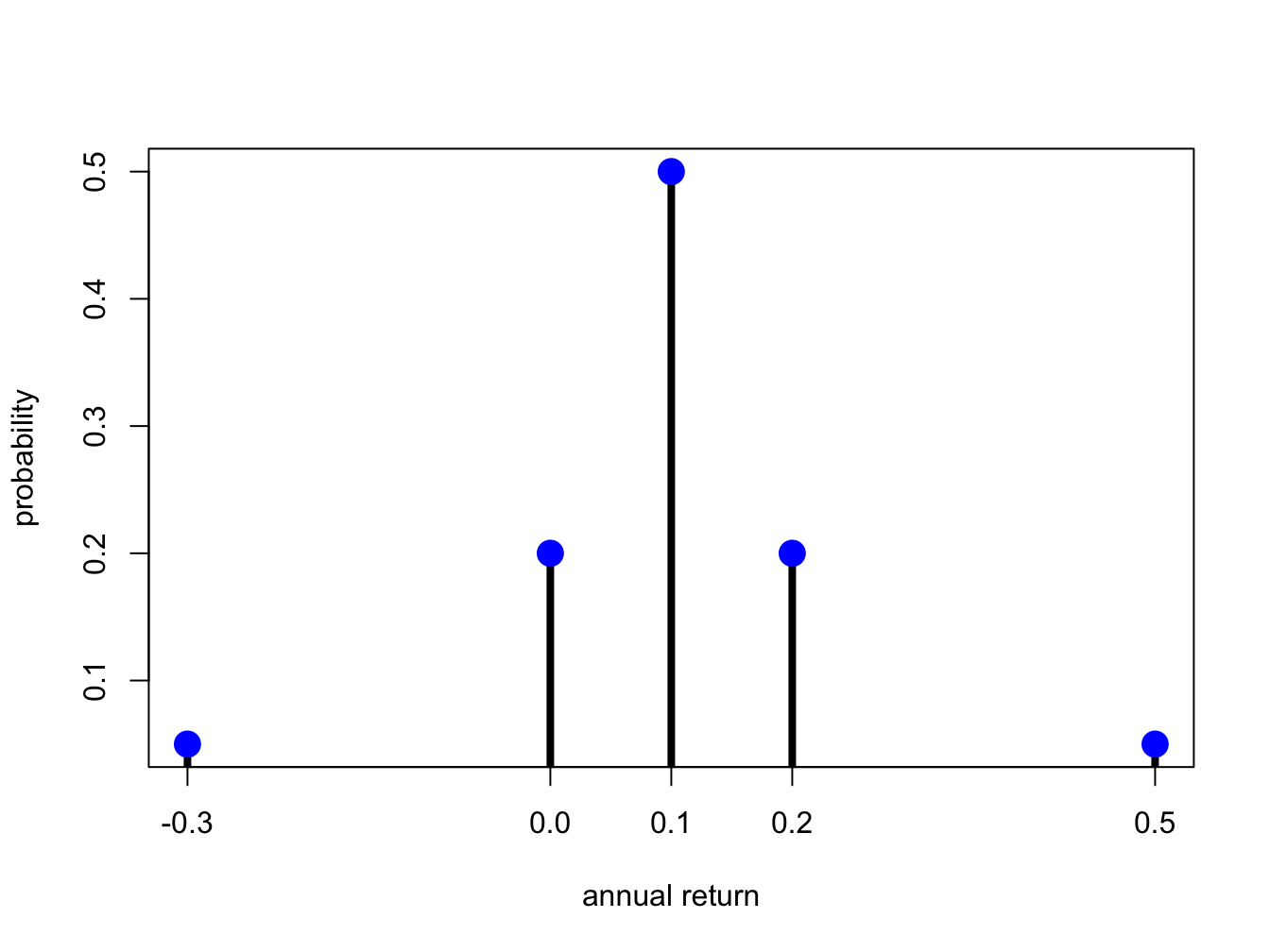
Figure 2.1: Discrete distribution for Microsoft stock.
The shape of the distribution is revealing. The center and most likely value is at \(0.1\) and the distribution is symmetric about this value (has the same shape to the left and to the right). Most of the probability is concentrated between \(0\) and \(0.2\) and there is very little probability associated with very large or small returns.
\(\blacksquare\)
2.1.1.1 The Bernoulli distribution
Let \(X=1\) if the price next month of Microsoft stock goes up and \(X=0\) if the price goes down (assuming it cannot stay the same). Then \(X\) is clearly a discrete random variable with sample space \(S_{X}=\{0,1\}\). If the probability of the stock price going up or down is the same then \(p(0)=p(1)=1/2\) and \(p(0)+p(1)=1\).
The probability distribution described above can be given an exact mathematical representation known as the Bernoulli distribution. Consider two mutually exclusive events generically called “success” and “failure”. For example, a success could be a stock price going up or a coin landing heads and a failure could be a stock price going down or a coin landing tails. The process creating the success or failure is called a Bernoulli trial. In general, let \(X=1\) if success occurs and let \(X=0\) if failure occurs. Let \(\Pr(X=1)=\pi\), where \(0<\pi<1\), denote the probability of success. Then \(\Pr(X=0)=1-\pi\) is the probability of failure. A mathematical model describing this distribution is: \[\begin{equation} p(x)=\Pr(X=x)=\pi^{x}(1-\pi)^{1-x},~x=0,1.\tag{2.1} \end{equation}\] When \(x=0\), \(p(0)=\pi^{0}(1-\pi)^{1-0}=1-\pi\) and when \(x=1,p(1)=\pi^{1}(1-\pi)^{1-1}=\pi\).
2.1.1.2 The binomial distribution
Consider a sequence of independent Bernoulli trials with success probability \(\pi\) generating a sequence of 0-1 variables indicating failures and successes. A binomial random variable \(X\) counts the number of successes in \(n\) Bernoulli trials, and is denoted \(X\sim B(n,\pi)\). The sample space is \(S_{X}=\{0,1,\ldots,n\}\) and: \[ \Pr(X=k)=\binom{n}{k}\pi^{k}(1-\pi)^{n-k}. \] The term \(\binom{n}{k}\) is the binomial coefficient, and counts the number of ways \(k\) objects can be chosen from \(n\) distinct objects. It is defined by: \[ \binom{n}{k}=\frac{n!}{(n-k)!k!}, \] where \(n!\) is the factorial of \(n\), or \(n(n-1)\cdots2\cdot1\).
2.1.2 Continuous random variables
A typical “bell-shaped” pdf is displayed in Figure 2.2 and the shaded area under the curve between -2 and 1 represents \(\Pr(-2\leq X \leq 1)\). For a continuous random variable, \(f(x)\neq\Pr(X=x)\) but rather gives the height of the probability curve at \(x\). In fact, \(\Pr(X=x)=0\) for all values of \(x\). That is, probabilities are not defined over single points. They are only defined over intervals. As a result, for a continuous random variable \(X\) we have: \[ \Pr(a\leq X\leq b)=\Pr(a<X\leq b)=\Pr(a<X<b)=\Pr(a\leq X<b). \]
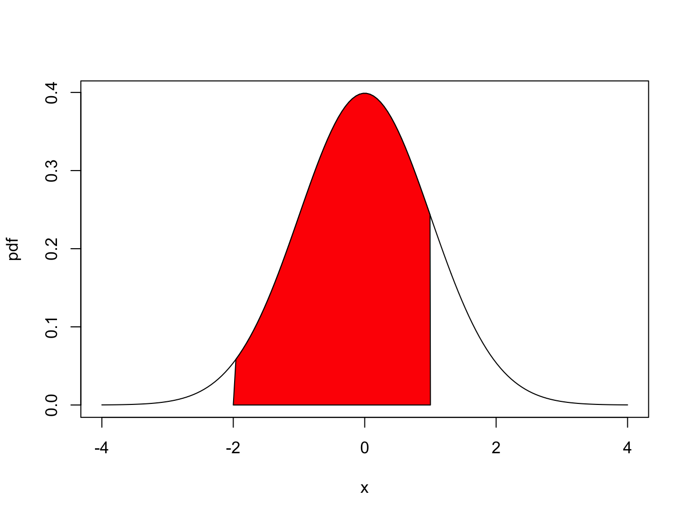
Figure 2.2: \(Pr(-2 \leq X \leq 1)\) is represented by the area under the probability curve.
2.1.2.1 The uniform distribution on an interval
Let \(X\) denote the annual return on Microsoft stock and let \(a\) and \(b\) be two real numbers such that \(a<b\). Suppose that the annual return on Microsoft stock can take on any value between \(a\) and \(b\). That is, the sample space is restricted to the interval \(S_{X}=\{x\in\mathcal{R}:a\leq x\leq b\}\). Further suppose that the probability that \(X\) will belong to any subinterval of \(S_{X}\) is proportional to the length of the interval. In this case, we say that \(X\) is uniformly distributed on the interval \([a,b]\). The pdf of \(X\) has a very simple mathematical form: \[ f(x)=\left\{ \begin{array}{c} \frac{1}{b-a}\\ 0 \end{array}\right.\begin{array}{c} \textrm{for }a\leq x\leq b,\\ \textrm{otherwise,} \end{array} \] and is presented graphically as a rectangle. It is easy to see that the area under the curve over the interval \([a,b]\) (area of rectangle) integrates to one: \[ \int_{a}^{b}\frac{1}{b-a}~dx=\frac{1}{b-a}\int_{a}^{b}~dx=\frac{1}{b-a}\left[x\right]_{a}^{b}=\frac{1}{b-a}[b-a]=1. \]
Let \(a=-1\) and \(b=1,\) so that \(b-a=2\). Consider computing the probability that \(X\) will be between -0.5 and 0.5. We solve: \[ \Pr(-0.5\leq X\leq0.5)=\int_{-0.5}^{0.5}\frac{1}{2}~dx=\frac{1}{2}\left[x\right]_{-0.5}^{0.5}=\frac{1}{2}\left[0.5-(-0.5)\right]=\frac{1}{2}. \] Next, consider computing the probability that the return will fall in the interval \([0,\delta]\) where \(\delta\) is some small number less than \(b=1\): \[ \Pr(0\leq X\leq\delta)=\frac{1}{2}\int_{0}^{\delta}dx=\frac{1}{2}[x]_{0}^{\delta}=\frac{1}{2}\delta. \] As \(\delta\rightarrow0\), \(\Pr(0\leq X\leq\delta)\rightarrow\Pr(X=0)\).
Using the above result we see that \[ \lim_{\delta\rightarrow0}\Pr(0\leq X\leq\delta)=\Pr(X=0)=\lim_{\delta\rightarrow0}\frac{1}{2}\delta=0. \] Hence, for continuous random variables probabilities are defined on intervals but not at distinct points.
\(\blacksquare\)
2.1.2.2 The standard normal distribution
The normal or Gaussian distribution is perhaps the most famous and most useful continuous distribution in all of statistics. The shape of the normal distribution is the familiar “bell curve”. As we shall see, it can be used to describe the probabilistic behavior of stock returns although other distributions may be more appropriate.
If a random variable \(X\) follows a standard normal distribution then we often write \(X\sim N(0,1)\) as short-hand notation. This distribution is centered at zero and has inflection points at \(\pm1\).10 The pdf of a standard normal random variable is given by: \[\begin{equation} f(x)=\frac{1}{\sqrt{2\pi}}\cdot e^{-\frac{1}{2}x^{2}},~-\infty\leq x\leq\infty.\tag{2.2} \end{equation}\] It can be shown via the change of variables formula in calculus that the area under the standard normal curve is one: \[ \int_{-\infty}^{\infty}\frac{1}{\sqrt{2\pi}}\cdot e^{-\frac{1}{2}x^{2}}dx=1. \] The standard normal distribution is illustrated in Figure 2.3. Notice that the distribution is symmetric about zero; i.e., the distribution has exactly the same form to the left and right of zero. Because the standard normal pdf formula is used so often it is given its own special symbol \(\phi(x)\).
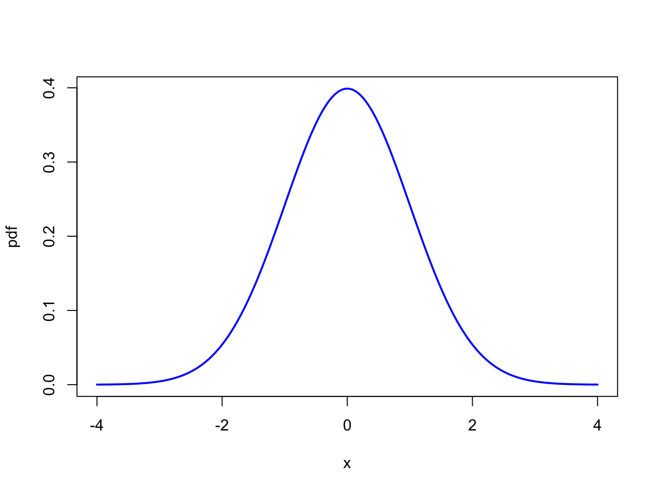
Figure 2.3: Standard normal density.
The normal distribution has the annoying feature that the area under the normal curve cannot be evaluated analytically. That is: \[ \Pr(a\leq X\leq b)=\int_{a}^{b}\frac{1}{\sqrt{2\pi}}\cdot e^{-\frac{1}{2}x^{2}}~dx, \] does not have a closed form solution. The above integral must be computed by numerical approximation. Areas under the normal curve, in one form or another, are given in tables in almost every introductory statistics book and standard statistical software can be used to find these areas. Some useful approximate results are: \[\begin{align*} \Pr(-1 & \leq X\leq1)\approx0.67,\\ \Pr(-2 & \leq X\leq2)\approx0.95,\\ \Pr(-3 & \leq X\leq3)\approx0.99. \end{align*}\]
2.1.3 The cumulative distribution function
The cdf has the following properties:
- If \(x_{1}<x_{2}\) then \(F_{X}(x_{1})\leq F_{X}(x_{2})\)
- \(F_{X}(-\infty)=0\) and \(F_{X}(\infty)=1\)
- \(\Pr(X>x)=1-F_{X}(x)\)
- \(\Pr(x_{1}<X\leq x_{2})=F_{X}(x_{2})-F_{X}(x_{1})\)
- \(F_{X}^{\prime}(x)=\frac{d}{dx}F_{X}(x)=f(x)\) if \(X\) is a continuous random variable and \(F_{X}(x)\) is continuous and differentiable.
The cdf for the discrete distribution of Microsoft from Table 2.1 is given by: \[ F_{X}(x)=\left\{ \begin{array}{c} 0,\\ 0.05,\\ 0.25,\\ 0.75\\ 0.95\\ 1 \end{array}\right.\begin{array}{c} x<-0.3\\ -0.3\leq x<0\\ 0\leq x<0.1\\ 0.1\leq x<0.2\\ 0.2\leq x<0.5\\ x>0.5 \end{array} \] and is illustrated in Figure 2.4.
\(\blacksquare\)
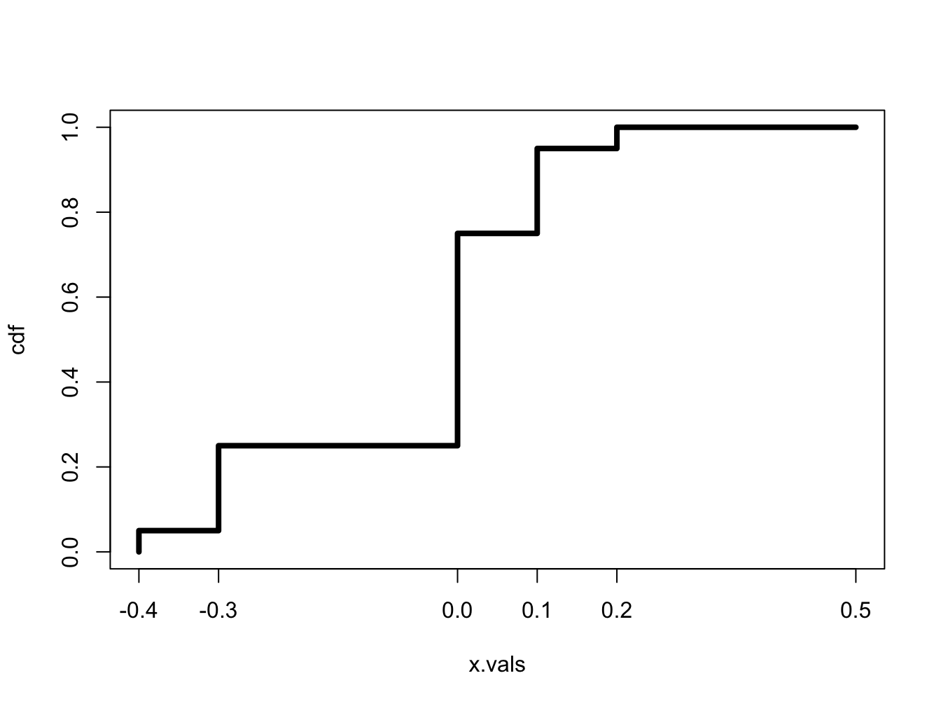
Figure 2.4: CDF of Discrete Distribution for Microsoft Stock Return.
The cdf for the uniform distribution over \([a,b]\) can be determined analytically: \[\begin{align*} F_{X}(x) & =\Pr(X<x)=\int_{-\infty}^{x}f(t)~dt\\ & =\frac{1}{b-a}\int_{a}^{x}~dt=\frac{1}{b-a}[t]_{a}^{x}=\frac{x-a}{b-a}. \end{align*}\] We can determine the pdf of \(X\) directly from the cdf via, \[ f(x)=F_{X}^{\prime}(x)=\frac{d}{dx}F_{X}(x)=\frac{1}{b-a}. \]
\(\blacksquare\)
The cdf of standard normal random variable \(X\) is used so often in statistics that it is given its own special symbol: \[\begin{equation} \Phi(x)=F_{X}(x)=\int_{-\infty}^{x}\frac{1}{\sqrt{2\pi}}e^{-\frac{1}{2}z^{2}}~dz.\tag{2.3} \end{equation}\] The cdf \(\Phi(x)\), however, does not have an analytic representation like the cdf of the uniform distribution and so the integral in (2.3) must be approximated using numerical techniques. A graphical representation of \(\Phi(x)\) is given in Figure 2.5. Because the standard normal pdf, \(\phi(x)\), is symmetric about zero and bell-shaped the standard normal CDF, \(\Phi(x)\), has an “S” shape where the middle of the “S” is at zero.
\(\blacksquare\)
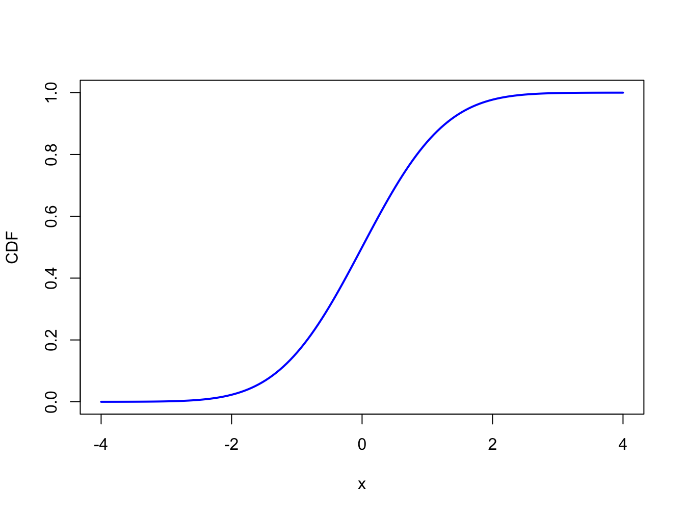
Figure 2.5: Standard normal cdf \(\Phi(x)\).
2.1.4 Quantiles of the distribution of a random variable
Definition 2.7 Consider a random variable \(X\) with continuous cdf \(F_{X}(x)\). For \(0\leq\alpha\leq1\), the \(100\cdot\alpha\%\) quantile of the distribution for \(X\) is the value \(q_{\alpha}\) that satisfies: \[ F_{X}(q_{\alpha})=\Pr(X\leq q_{\alpha})=\alpha. \] For example, the 5% quantile of \(X\), \(q_{0.05}\), satisfies, \[ F_{X}(q_{0.05})=\Pr(X\leq q_{0.05})=0.05. \]
The median of the distribution is the 50% quantile. That is, the median, \(q_{0.5}\), satisfies, \[ F_{X}(q_{0.5})=\Pr(X\leq q_{0.5})=0.5. \]
If \(F_{X}\) is invertible then \(q_{\alpha}\) may be determined analytically as: \[\begin{equation} q_{\alpha}=F_{X}^{-1}(\alpha)\tag{2.4} \end{equation}\] where \(F_{X}^{-1}\) denotes the inverse function of \(F_{X}\).11 Hence, the 5% quantile and the median may be determined from \[ q_{0.05}=F_{X}^{-1}(.05),q_{0.5}=F_{X}^{-1}(.5). \] The inverse cdf \(F_{X}^{-1}\) is sometimes called the quantile function.
Let \(X\sim U[a,b]\) where \(b>a\). Recall, the cdf of \(X\) is given by: \[ F_{X}(x)=\frac{x-a}{b-a},~a\leq x\leq b, \] which is continuous and strictly increasing. Given \(\alpha\in[0,1]\) such that \(F_{X}(x)=\alpha\), solving for \(x\) gives the inverse cdf: \[\begin{equation} x=F_{X}^{-1}(\alpha)=\alpha(b-a)+a.\tag{2.5} \end{equation}\] Using (2.5), the 5% quantile and median, for example, are given by: \[\begin{align*} q_{0.05} & =F_{X}^{-1}(.05)=.05(b-a)+a=.05b+.95a,\\ q_{0.5} & =F_{X}^{-1}(.5)=.5(b-a)+a=.5(a+b). \end{align*}\] If \(a=0\) and \(b=1\), then \(q_{0.05}=0.05\) and \(q_{0.5}=0.5\).
\(\blacksquare\)
Let \(X\sim N(0,1).\) The quantiles of the standard normal distribution are determined by solving \[\begin{equation} q_{\alpha}=\Phi^{-1}(\alpha),\tag{2.6} \end{equation}\] where \(\Phi^{-1}\) denotes the inverse of the cdf \(\Phi\). This inverse function must be approximated numerically and is available in most spreadsheets and statistical software. Using the numerical approximation to the inverse function, the 1%, 2.5%, 5%, 10% quantiles and median are given by: \[\begin{align*} q_{0.01} & =\Phi^{-1}(.01)=-2.33,~q_{0.025}=\Phi^{-1}(.025)=-1.96,\\ q_{0.05} & =\Phi^{-1}(.05)=-1.645,~q_{0.10}=\Phi^{-1}(.10)=-1.28,\\ q_{0.5} & =\Phi^{-1}(.5)=0. \end{align*}\] Often, the standard normal quantile is denoted \(z_{\alpha}\).
\(\blacksquare\)
2.1.5 R functions for discrete and continuous distributions
R has built-in functions for a number of discrete and continuous distributions
that are commonly used in probability modeling and statistical analysis.
These are summarized in Table 2.2.
For each distribution, there are four functions starting with d,
p, q, and r that compute density
(pdf) values, cumulative probabilities (cdf), quantiles
(inverse cdf) and random draws, respectively. Consider, for
example, the functions associated with the normal distribution. The
functions dnorm(), pnorm() and qnorm()
evaluate the standard normal density (2.2),
the cdf (2.3), and the inverse cdf or quantile
function (2.6), respectively, with
the default values mean = 0 and sd = 1. The function
rnorm() returns a specified number of simulated values from
the normal distribution.
| Distribution | Function (root) | Parameters | Defaults |
|---|---|---|---|
| beta | beta |
shape1, shape2 | _, _ |
| binomial | binom |
size, prob | _, _ |
| cauchy | cauchy |
location, scale | 0, 1 |
| chi-squared | chisq |
df, ncp | _, 1 |
| F | f |
df1, df2 | _, _ |
| gamma | gamma |
shape, rate, scale | _, 1, 1/rate |
| geometric | geom |
prob | _ |
| hyper-geometric | hyper |
m, n, k | _, _, _ |
| log-normal | lnorm |
meanlog, sdlog | 0, 1 |
| logistic | logis |
location, scale | 0, 1 |
| negative binomial | nbinom |
size, prob, mu | _,_,_ |
| normal | norm |
mean, sd | 0, 1 |
| Poisson | pois |
Lambda | 1 |
| Student’s t | t |
df, ncp | _, 1 |
| uniform | unif |
min, max | 0, 1 |
| Weibull | weibull |
shape, scale | _, 1 |
| Wilcoxon | wilcoxon |
m, n | _, _ |
Commonly used distributions used in finance application are the binomial, chi-squared, log normal, normal, and Student’s t.
2.1.5.1 Finding areas under the standard normal curve
Let \(X\) denote a standard normal random variable. Given that the total area under the normal curve is one and the distribution is symmetric about zero, the following results hold:
- \(\Pr(X\leq z)=1-\Pr(X\geq z)\) and \(\Pr(X\geq z)=1-\Pr(X\leq z)\)
- \(\Pr(X\geq z)=\Pr(X\leq-z)\)
- \(\Pr(X\geq0)=\Pr(X\leq0)=0.5\)
The following examples show how to do probability calculations with standard normal random variables.
First, consider finding \(\Pr(X\geq2)\). By the symmetry of the normal distribution, \(\Pr(X\geq2)=\Pr(X\leq-2)=\Phi(-2)\). In R use:
## [1] 0.02275Next, consider finding \(\Pr(-1\leq X\leq2)\). Using the cdf, we compute \(\Pr(-1\leq X\leq2)=\Pr(X\leq2)-\Pr(X\leq-1)=\Phi(2)-\Phi(-1)\). In R use:
## [1] 0.8186Finally, using R the exact values for \(\Pr(-1\leq X\leq1)\), \(\Pr(-2\leq X\leq2)\) and \(\Pr(-3\leq X\leq3)\) are:
## [1] 0.6827## [1] 0.9545## [1] 0.9973\(\blacksquare\)
2.1.5.2 Plotting distributions
When working with a probability distribution, it is a good idea to make plots of the pdf or cdf to reveal important characteristics. The following examples illustrate plotting distributions using R.
The graphs of the standard normal pdf and cdf in Figures 2.3 and 2.5 were created using the following R code:
# plot pdf
x.vals = seq(-4, 4, length=150)
plot(x.vals, dnorm(x.vals), type="l", lwd=2, col="blue",
     xlab="x", ylab="pdf")
# plot cdf
plot(x.vals, pnorm(x.vals), type="l", lwd=2, col="blue",
     xlab="x", ylab="CDF")
\(\blacksquare\)
Figure 2.2 showing \(\Pr(-2\leq X\leq1)\) as a red shaded area is created with the following code:
lb = -2
ub = 1
x.vals = seq(-4, 4, length=150)
d.vals = dnorm(x.vals)
# plot normal density
plot(x.vals, d.vals, type="l", xlab="x", ylab="pdf")
i = x.vals >= lb & x.vals <= ub
# add shaded region between -2 and 1
polygon(c(lb, x.vals[i], ub), c(0, d.vals[i], 0), col="red")
\(\blacksquare\)
2.1.6 Shape characteristics of probability distributions
Very often we would like to know certain shape characteristics of a probability distribution. We might want to know where the distribution is centered, and how spread out the distribution is about the central value. We might want to know if the distribution is symmetric about the center or if the distribution has a long left or right tail. For stock returns we might want to know about the likelihood of observing extreme values for returns representing market crashes. This means that we would like to know about the amount of probability in the extreme tails of the distribution. In this section we discuss four important shape characteristics of a probability distribution:
- expected value (mean): measures the center of mass of a distribution
- variance and standard deviation (volatility): measures the spread about the mean
- skewness: measures symmetry about the mean
- kurtosis: measures “tail thickness”
2.1.6.1 Expected Value
The expected value of a random variable \(X,\) denoted \(E[X]\) or \(\mu_{X}\), measures the center of mass of the pdf.
Equation (2.7) shows that \(E[X]\) is a probability weighted average of the possible values of \(X\).
Using the discrete distribution for the return on Microsoft stock in Table 2.1, the expected return is computed as: \[\begin{align*} E[X] =&(-0.3)\cdot(0.05)+(0.0)\cdot(0.20)+(0.1)\cdot(0.5)\\ &+(0.2)\cdot(0.2)+(0.5)\cdot(0.05)\\ =&0.10. \end{align*}\]
\(\blacksquare\)
Let \(X\) be a Bernoulli random variable with success probability \(\pi\). Then, \[ E[X]=0\cdot(1-\pi)+1\cdot\pi=\pi. \] That is, the expected value of a Bernoulli random variable is its probability of success. Now, let \(Y\sim B(n,\pi)\). It can be shown that: \[\begin{equation} E[Y]=\sum_{k=0}^{n}k\binom{n}{k}\pi^{k}(1-\pi)^{n-k}=n\pi.\tag{2.8} \end{equation}\]
\(\blacksquare\)
Definition 2.9 For a continuous random variable \(X\) with pdf \(f(x)\), the expected value is defined as: \[\begin{equation} \mu_{X}=E[X]=\int_{-\infty}^{\infty}x\cdot f(x)~dx.\tag{2.9} \end{equation}\]
Suppose \(X\) has a uniform distribution over the interval \([a,b]\). Then, \[\begin{align*} E[X] & =\frac{1}{b-a}\int_{a}^{b}x~dx=\frac{1}{b-a}\left[\frac{1}{2}x^{2}\right]_{a}^{b}\\ & =\frac{1}{2(b-a)}\left[b^{2}-a^{2}\right]\\ & =\frac{(b-a)(b+a)}{2(b-a)}=\frac{b+a}{2}. \end{align*}\] If \(b=-1\) and \(a=1\), then \(E[X]=0\).
\(\blacksquare\)
Let \(X\sim N(0,1)\). Then it can be shown that: \[ E[X]=\int_{-\infty}^{\infty}x\cdot\frac{1}{\sqrt{2\pi}}e^{-\frac{1}{2}x^{2}}~dx=0. \] Hence, the standard normal distribution is centered at zero.
\(\blacksquare\)
2.1.6.2 Expectation of a function of a random variable
The other shape characteristics of the distribution of a random variable \(X\) are based on expectations of certain functions of \(X\).
2.1.6.3 Variance and standard deviation
The variance of a random variable \(X\), denoted \(\mathrm{var}(X)\) or \(\sigma_{X}^{2}\), measures the spread of the distribution about the mean using the function \(g(X)=(X-\mu_{X})^{2}\). If most values of \(X\) are close to \(\mu_{X}\) then on average \((X-\mu_{X})^{2}\) will be small. In contrast, if many values of \(X\) are far below and/or far above \(\mu_{X}\) then on average \((X-\mu_{X})^{2}\) will be large. Squaring the deviations about \(\mu_{X}\) guarantees a positive value.
Definition 2.11 For a discrete or continuous random variable \(X\), the variance and standard deviation of \(X\) are defined as: \[\begin{align} \sigma_{X}^{2}&=\mathrm{var}(X)=E[(X-\mu_{X})^{2}],\tag{2.12} \\ \sigma_{X} &= \mathrm{sd}(X)= \sqrt{\sigma_{X}^{2}} = \sigma_{X}. \tag{2.13} \end{align}\]
Because \(\sigma_{X}^{2}\) represents an average squared deviation, it is not in the same units as \(X\). The standard deviation of \(X\) is the square root of the variance and is in the same units as \(X\). For “bell-shaped” distributions, \(\sigma_{X}\) measures the typical size of a deviation from the mean value.
The computation of (2.12) can often be simplified by using the result: \[\begin{equation} \mathrm{var}(X)=E[(X-\mu_{X})^{2}]=E[X^{2}]-\mu_{X}^{2}\tag{2.14} \end{equation}\] We will learn how to derive this result later in the chapter.
Using the discrete distribution for the return on Microsoft stock in Table 2.1 and the result that \(\mu_{X}=0.1\), we have: \[\begin{align*} \mathrm{var}(X) & =(-0.3-0.1)^{2}\cdot(0.05)+(0.0-0.1)^{2}\cdot(0.20)+(0.1-0.1)^{2}\cdot(0.5)\\ & +(0.2-0.1)^{2}\cdot(0.2)+(0.5-0.1)^{2}\cdot(0.05)\\ & =0.020. \end{align*}\] Alternatively, we can compute \(\mathrm{var}(X)\) using (2.14): \[\begin{align*} E[X^{2}]-\mu_{X}^{2} & =(-0.3)^{2}\cdot(0.05)+(0.0)^{2}\cdot(0.20)+(0.1)^{2}\cdot(0.5)\\ & +(0.2)^{2}\cdot(0.2)+(0.5)^{2}\cdot(0.05)-(0.1)^{2}\\ & =0.020. \end{align*}\] The standard deviation is \(\sqrt{0.020}=0.141\). Given that the distribution is fairly bell-shaped we can say that typical values deviate from the mean value of \(10\%\) by about \(\pm 14.1\%\).
\(\blacksquare\)
Let \(X\) be a Bernoulli random variable with success probability \(\pi\). Given that \(\mu_{X}=\pi\) it follows that: \[\begin{align*} \mathrm{var}(X) & =(0-\pi)^{2}\cdot(1-\pi)+(1-\pi)^{2}\cdot\pi\\ & =\pi^{2}(1-\pi)+(1-\pi)^{2}\pi\\ & =\pi(1-\pi)\left[\pi+(1-\pi)\right]\\ & =\pi(1-\pi),\\ \mathrm{sd}(X) & =\sqrt{\pi(1-\pi)}. \end{align*}\] Now, let \(Y\sim B(n,\pi)\): It can be shown that: \[ \mathrm{var}(Y)=n\pi(1-\pi) \] and so \(\mathrm{sd}(Y)=\sqrt{n\pi(1-\pi)}\).
\(\blacksquare\)
Let \(X\sim U[a,b]\). Using (2.14) and \(\mu_{X}=\frac{a+b}{2}\), after some algebra, it can be shown that: \[ \mathrm{var}(X)=E[X^{2}]-\mu_{X}^{2}=\frac{1}{b-a}\int_{a}^{b}x^{2}~dx-\left(\frac{a+b}{2}\right)^{2}=\frac{1}{12}(b-a)^{2}, \] and \(\mathrm{sd}(X)=(b-a)/\sqrt{12}\).
\(\blacksquare\)
Let \(X\sim N(0,1)\). Here, \(\mu_{X}=0\) and it can be shown that: \[ \sigma_{X}^{2}=\int_{-\infty}^{\infty}x^{2}\cdot\frac{1}{\sqrt{2\pi}}e^{-\frac{1}{2}x^{2}}~dx=1. \] It follows that sd\((X)=1\).
\(\blacksquare\)
2.1.6.4 The general normal distribution
Recall, if \(X\) has a standard normal distribution then \(E[X]=0\), \(\mathrm{var}(X)=1\). A general normal random variable \(X\) has \(E[X]=\mu_{X}\) and \(\mathrm{var}(X)=\sigma_{X}^{2}\) and is denoted \(X\sim N(\mu_{X},\sigma_{X}^{2})\). Its pdf is given by: \[\begin{equation} f(x)=\frac{1}{\sqrt{2\pi\sigma_{X}^{2}}}\exp\left\{ -\frac{1}{2\sigma_{X}^{2}}\left(x-\mu_{X}\right)^{2}\right\} ,~-\infty\leq x\leq\infty.\tag{2.15} \end{equation}\] Showing that \(E[X]=\mu_{X}\) and \(\mathrm{var}(X)=\sigma_{X}^{2}\) is a bit of work and is good calculus practice. As with the standard normal distribution, areas under the general normal curve cannot be computed analytically. Using numerical approximations, it can be shown that: \[\begin{align*} \Pr(\mu_{X}-\sigma_{X} & <X<\mu_{X}+\sigma_{X})\approx0.67,\\ \Pr(\mu_{X}-2\sigma_{X} & <X<\mu_{X}+2\sigma_{X})\approx0.95,\\ \Pr(\mu_{X}-3\sigma_{X} & <X<\mu_{X}+3\sigma_{X})\approx0.99. \end{align*}\] Hence, for a general normal random variable about 95% of the time we expect to see values within \(\pm\) 2 standard deviations from its mean. Observations more than three standard deviations from the mean are very unlikely.
Let \(R\) denote the monthly return on an investment in Microsoft stock, and assume that it is normally distributed with mean \(\mu_{R}=0.01\) and standard deviation \(\sigma_{R}=0.10\). That is, \(R\sim N(0.01,(0.10)^{2})\). Notice that \(\sigma_{R}^{2}=0.01\) and is not in units of return per month. Figure 2.6 illustrates the distribution and is created using:
mu.r = 0.01
sd.r = 0.1
x.vals = seq(-4, 4, length=150)*sd.r + mu.r
plot(x.vals, dnorm(x.vals, mean=mu.r, sd=sd.r), type="l", lwd=2,
     col="blue", xlab="x", ylab="pdf")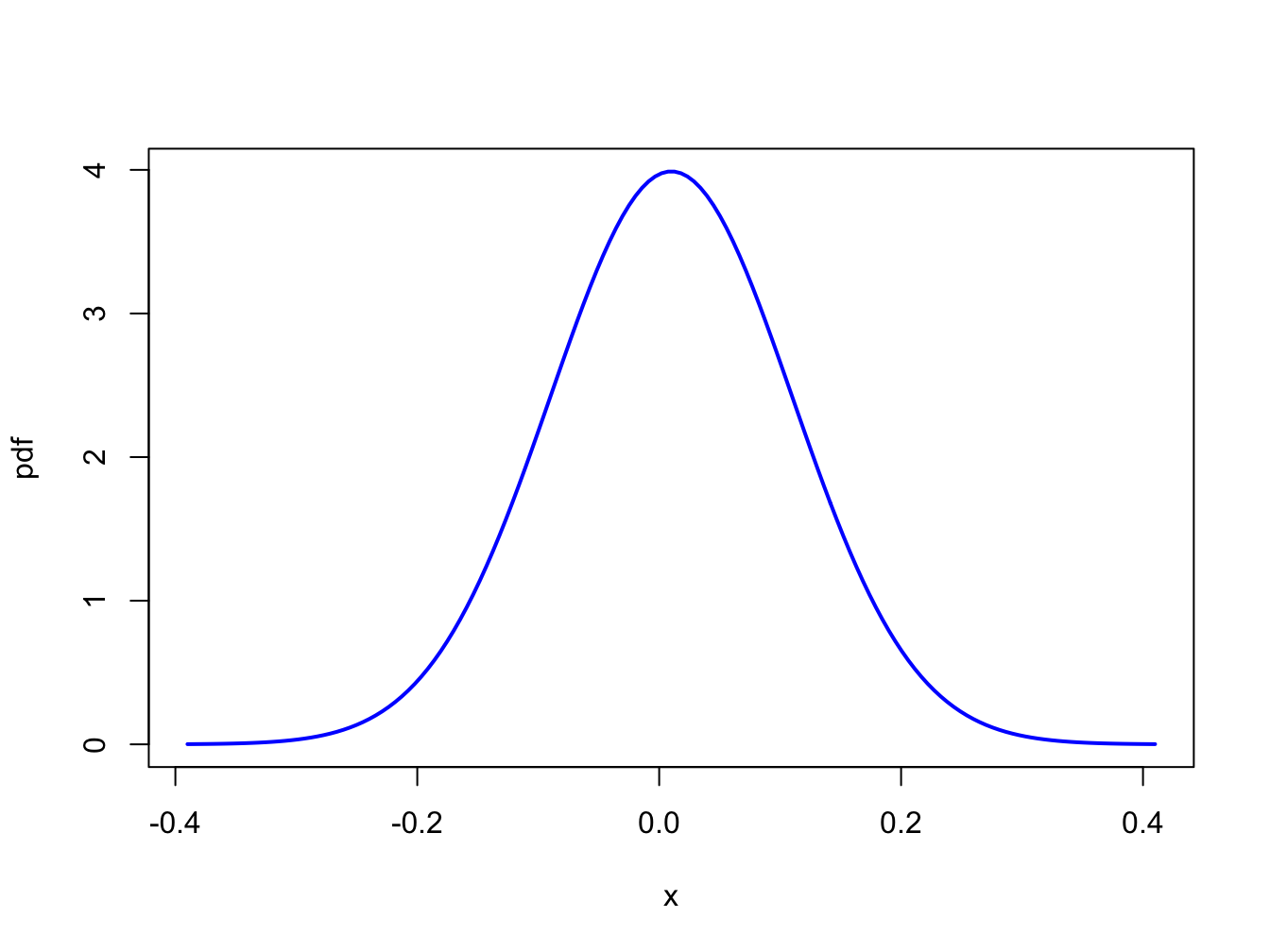
Figure 2.6: Normal distribution for the monthly returns on Microsoft: \(R\sim N(0.01,(0.10)^{2})\).
Notice that essentially all of the probability lies between \(-0.3\)
and \(0.3\). Using the R function pnorm(), we can easily compute
the probabilities \(\Pr(R<-0.5)\), \(\Pr(R<0)\), \(\Pr(R>0.5)\) and \(\Pr(R>1)\):
## [1] 1.698e-07## [1] 0.4602## [1] 4.792e-07## [1] 0Using the R function , we can find the quantiles \(q_{0.01}\), \(q_{0.05}\), \(q_{0.95}\) and \(q_{0.99}\):
## [1] -0.2226 -0.1545 0.1745 0.2426Hence, over the next month, there are 1% and 5% chances of losing more than 22.2% and 15.5%, respectively. In addition, there are 5% and 1% chances of gaining more than 17.5% and 24.3%, respectively.
\(\blacksquare\)
Consider the following investment problem. We can invest in two non-dividend paying stocks, Amazon and Boeing, over the next month. Let \(R_{A}\) denote the monthly return on Amazon and \(R_{B}\) denote the monthly return on Boeing. Assume that \(R_{A}\sim N(0.02,(0.10)^{2})\) and \(R_{B}\sim N(0.01,(0.05)^{2})\). Figure 2.7 shows the pdfs for the two returns. Notice that \(\mu_{A}=0.02>\mu_{B}=0.01\) but also that \(\sigma_{A}=0.10>\sigma_{B}=0.05\). The return we expect on Amazon is bigger than the return we expect on Boeing but the variability of Amazon’s return is also greater than the variability of Boeing’s return. The high return variability (volatility) of Amazon reflects the higher risk associated with investing in Amazon compared to investing in Boeing. If we invest in Boeing we get a lower expected return, but we also get less return variability or risk. For example, the probability of losing more than \(10\%\) in one month for Amazon is
## [1] 0.1151and the probability of losing more than \(10\%\) in one month for Boeing is
## [1] 0.0139Of course, there is also a higher probability for upside return for Amazon than for Boeing. This example illustrates the fundamental “no free lunch” principle of economics and finance: you can’t get something for nothing. In general, to get a higher expected return you must be prepared to take on higher risk.
\(\blacksquare\)
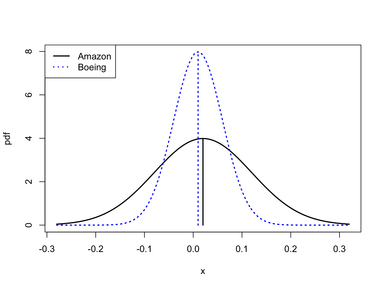
Figure 2.7: Risk-return tradeoff between one-month investments in Amazon and Boeing stock.
Let \(R_{t}\) denote the simple annual return on an asset, and suppose that \(R_{t}\sim N(0.05,(0.50)^{2})\). Because asset prices must be non-negative, \(R_{t}\) must always be larger than \(-1\). However, the normal distribution is defined for \(-\infty\leq R_{t}\leq\infty\) and based on the assumed normal distribution \(\Pr(R_{t}<-1)=0.018\). That is, there is a 1.8% chance that \(R_{t}\) is smaller than \(-1\). This implies that there is a 1.8% chance that the asset price at the end of the year will be negative! This is one reason why the normal distribution may not be appropriate for simple returns.
\(\blacksquare\)
Let \(r_{t}=\ln(1+R_{t})\) denote the continuously compounded annual return on an asset, and suppose that \(r_{t}\sim N(0.05,(0.50)^{2})\). Unlike the simple return, the continuously compounded return can take on values less than \(-1\). In fact, \(r_{t}\) is defined for \(-\infty\leq r_{t}\leq\infty\). For example, suppose \(r_{t}=-2\). This implies a simple return of \(R_{t}=e^{-2}-1=-0.865\). Then \(\Pr(r_{t}\leq-2)=\Pr(R_{t}\leq-0.865)=0.00002\). Although the normal distribution allows for values of \(r_{t}\) smaller than \(-1\), the implied simple return \(R_{t}\) will always be greater than \(-1\).
\(\blacksquare\)
2.1.6.5 The Log-Normal Distribution
Let \(X\) \(\sim N(\mu_{X},\sigma_{X}^{2})\), which is defined for \(-\infty<X<\infty\). The log-normally distributed random variable \(Y\) is determined from the normally distributed random variable \(X\) using the transformation \(Y=e^{X}\). In this case, we say that \(Y\) is log-normally distributed and write: \[\begin{equation} Y\sim\ln N(\mu_{X},\sigma_{X}^{2}),~0<Y<\infty.\tag{2.16} \end{equation}\] The pdf of the log-normal distribution for \(Y\) can be derived from the normal distribution for \(X\) using the change-of-variables formula from calculus and is given by: \[\begin{equation} f(y)=\frac{1}{y\sigma_{X}\sqrt{2\pi}}e^{-\frac{(\ln y-\mu_{X})^{2}}{2\sigma_{X}^{2}}}.\tag{2.17} \end{equation}\] Due to the exponential transformation, \(Y\) is only defined for non-negative values. It can be shown that: \[\begin{align} \mu_{Y} & =E[Y]=e^{\mu_{X}+\sigma_{X}^{2}/2},\tag{2.18}\\ \sigma_{Y}^{2} & =\mathrm{var}(Y)=e^{2\mu_{X}+\sigma_{X}^{2}}(e^{\sigma_{X}^{2}}-1).\nonumber \end{align}\]
Let \(r_{t}=\ln(P_{t}/P_{t-1})\) denote the continuously compounded monthly return on an asset and assume that \(r_{t}\sim N(0.05,(0.50)^{2})\). That is, \(\mu_{r}=0.05\) and \(\sigma_{r}=0.50\). Let \(R_{t}=(P_{t}-P_{t-1})/P_{t}\) denote the simple monthly return. The relationship between \(r_{t}\) and \(R_{t}\) is given by \(r_{t}=\ln(1+R_{t})\) and \(1+R_{t}=e^{r_{t}}\). Since \(r_{t}\) is normally distributed, \(1+R_{t}\) is log-normally distributed. Notice that the distribution of \(1+R_{t}\) is only defined for positive values of \(1+R_{t}\). This is appropriate since the smallest value that \(R_{t}\) can take on is \(-1\). Using (2.18), the mean and variance for \(1+R_{t}\) are given by: \[\begin{align*} \mu_{1+R} & =e^{0.05+(0.5)^{2}/2}=1.191\\ \sigma_{1+R}^{2} & =e^{2(0.05)+(0.5)^{2}}(e^{(0.5)^{2}}-1)=0.563 \end{align*}\] The pdfs for \(r_{t}\) and \(R_{t}\) are shown in Figure 2.8.
\(\blacksquare\)
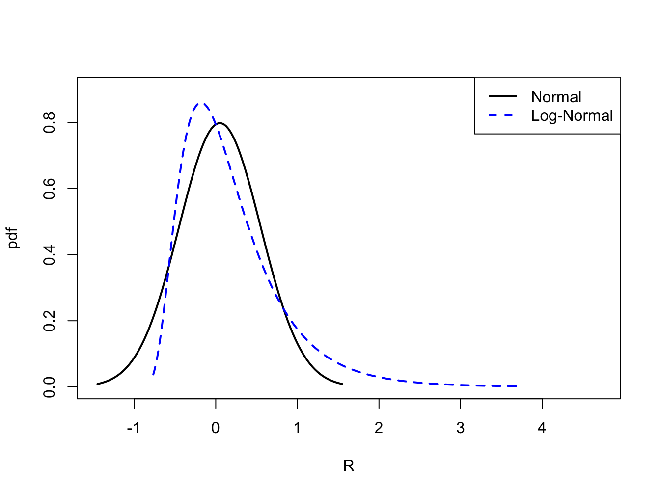
Figure 2.8: Normal distribution for \(r_{t}\) and log-normal distribution for \(R_{t}=e^{r_{t}}-1\).
2.1.6.6 Skewness
Definition 2.12 The skewness of a random variable \(X\), denoted \(\mathrm{skew}(X)\), measures the symmetry of a distribution about its mean value using the function \(g(X)=(X-\mu_{X})^{3}/\sigma_{X}^{3}\), where \(\sigma_{X}^{3}\) is just \(\mathrm{sd}(X)\) raised to the third power: \[\begin{equation} \mathrm{skew}(X)=\frac{E[(X-\mu_{X})^{3}]}{\sigma_{X}^{3}}\tag{2.19} \end{equation}\]
When \(X\) is far below its mean, \((X-\mu_{X})^{3}\) is a big negative number. When \(X\) is far above its mean, \((X-\mu_{X})^{3}\) is a big positive number. Hence, if there are more big values of \(X\) below \(\mu_{X}\) then \(\mathrm{skew}(X)<0\). Conversely, if there are more big values of \(X\) above \(\mu_{X}\) then \(\mathrm{skew}(X)>0\). If \(X\) has a symmetric distribution, then \(\mathrm{skew}(X)=0\) since positive and negative values in (2.19) cancel out. If \(\mathrm{skew}(X)>0\), then the distribution of \(X\) has a long right tail and if \(\mathrm{skew}(X)<0\) the distribution of \(X\) has a long left tail. These cases are illustrated in Figure 2.9.
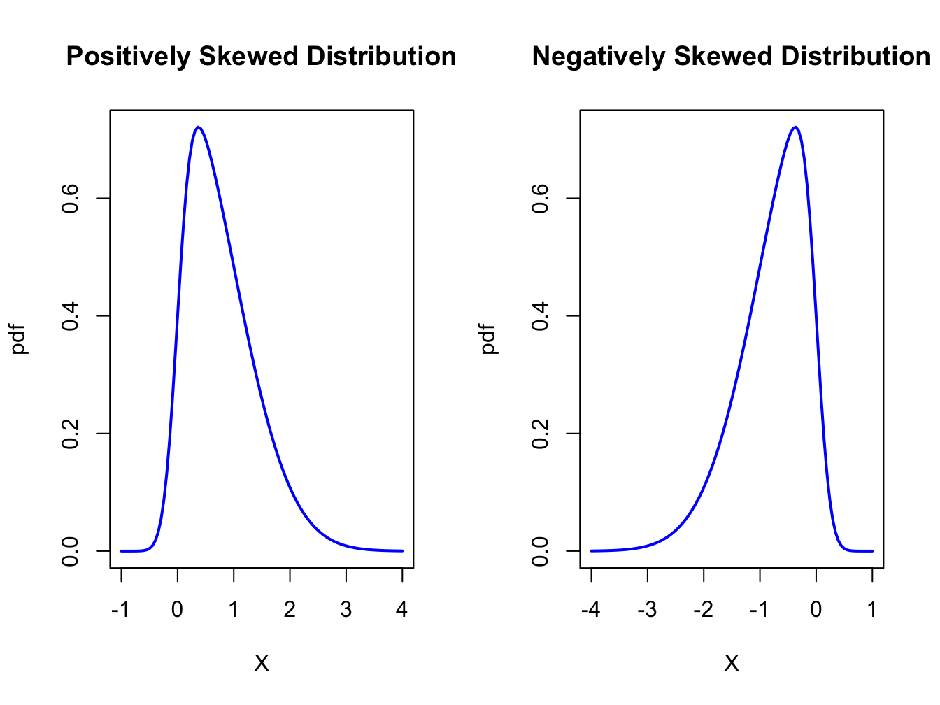
Figure 2.9: Skewed distributions.
Using the discrete distribution for the return on Microsoft stock in Table 2.1, the results that \(\mu_{X}=0.1\) and \(\sigma_{X}=0.141\), we have: \[\begin{align*} \mathrm{skew}(X) & =[(-0.3-0.1)^{3}\cdot(0.05)+(0.0-0.1)^{3}\cdot(0.20)+(0.1-0.1)^{3}\cdot(0.5)\\ & +(0.2-0.1)^{3}\cdot(0.2)+(0.5-0.1)^{3}\cdot(0.05)]/(0.141)^{3}\\ & =0.0. \end{align*}\]
\(\blacksquare\)
Suppose \(X\) has a general normal distribution with mean \(\mu_{X}\) and variance \(\sigma_{X}^{2}\). Then it can be shown that: \[ \mathrm{skew}(X)=\int_{-\infty}^{\infty}\frac{(x-\mu_{X})^{3}}{\sigma_{X}^{3}}\cdot\frac{1}{\sqrt{2\pi\sigma^{2}}}e^{-\frac{1}{2\sigma_{X}^{2}}\left(x-\mu_{X}\right)^{2}}~dx=0. \] This result is expected since the normal distribution is symmetric about it’s mean value \(\mu_{X}\).
\(\blacksquare\)
Let \(Y=e^{X},\) where \(X\sim N(\mu_{X},\sigma_{X}^{2})\), be a log-normally distributed random variable with parameters \(\mu_{X}\) and \(\sigma_{X}^{2}\). Then it can be shown that: \[ \mathrm{skew}(Y)=\left(e^{\sigma_{X}^{2}}+2\right)\sqrt{e^{\sigma_{X}^{2}}-1}>0. \] Notice that \(\mathrm{skew}(Y)\) is always positive, indicating that the distribution of \(Y\) has a long right tail, and that it is an increasing function of \(\sigma_{X}^{2}\). This positive skewness is illustrated in Figure 2.8.
\(\blacksquare\)
2.1.6.7 Kurtosis
Definition 2.13 The kurtosis of a random variable \(X\), denoted \(\mathrm{kurt}(X)\), measures the thickness in the tails of a distribution and is based on \(g(X)=(X-\mu_{X})^{4}/\sigma_{X}^{4}\): \[\begin{equation} \mathrm{kurt}(X)=\frac{E[(X-\mu_{X})^{4}]}{\sigma_{X}^{4}},\tag{2.20} \end{equation}\] where \(\sigma_{X}^{4}\) is just \(\mathrm{sd}(X)\) raised to the fourth power.
Since kurtosis is based on deviations from the mean raised to the fourth power, large deviations get lots of weight. Hence, distributions with large kurtosis values are ones where there is the possibility of extreme values. In contrast, if the kurtosis is small then most of the observations are tightly clustered around the mean and there is very little probability of observing extreme values.
Using the discrete distribution for the return on Microsoft stock in Table 2.1, the results that \(\mu_{X}=0.1\) and \(\sigma_{X}=0.141\), we have: \[\begin{align*} \mathrm{kurt}(X) & =[(-0.3-0.1)^{4}\cdot(0.05)+(0.0-0.1)^{4}\cdot(0.20)+(0.1-0.1)^{4}\cdot(0.5)\\ & +(0.2-0.1)^{4}\cdot(0.2)+(0.5-0.1)^{4}\cdot(0.05)]/(0.141)^{4}\\ & =6.5. \end{align*}\]
\(\blacksquare\)
Suppose \(X\) has a general normal distribution with mean \(\mu_{X}\) and variance \(\sigma_{X}^{2}\). Then it can be shown that: \[ \mathrm{kurt}(X)=\int_{-\infty}^{\infty}\frac{(x-\mu_{X})^{4}}{\sigma_{X}^{4}}\cdot\frac{1}{\sqrt{2\pi\sigma_{X}^{2}}}e^{-\frac{1}{2}(\frac{x-\mu_{X}}{\sigma_{X}})^{2}}~dx=3. \] Hence, a kurtosis of 3 is a benchmark value for tail thickness of bell-shaped distributions. If a distribution has a kurtosis greater than 3, then the distribution has thicker tails than the normal distribution. If a distribution has kurtosis less than 3, then the distribution has thinner tails than the normal.
\(\blacksquare\)
Sometimes the kurtosis of a random variable is described relative to the kurtosis of a normal random variable. This relative value of kurtosis is referred to as excess kurtosis and is defined as: \[\begin{equation} \mathrm{ekurt}(X)=\mathrm{kurt}(X)-3\tag{2.21} \end{equation}\] If the excess kurtosis of a random variable is equal to zero then the random variable has the same kurtosis as a normal random variable. If excess kurtosis is greater than zero, then kurtosis is larger than that for a normal; if excess kurtosis is less than zero, then kurtosis is less than that for a normal.
2.1.6.8 The Student’s t Distribution
The kurtosis of a random variable gives information on the tail thickness of its distribution. The normal distribution, with kurtosis equal to three, gives a benchmark for the tail thickness of symmetric distributions. A distribution similar to the standard normal distribution but with fatter tails, and hence larger kurtosis, is the Student’s t distribution. If \(X\) has a Student’s t distribution with degrees of freedom parameter \(v\), denoted \(X\sim t_{v},\) then its pdf has the form: \[\begin{equation} f(x)=\frac{\Gamma\left(\frac{v+1}{2}\right)}{\sqrt{v\pi}\Gamma\left(\frac{v}{2}\right)}\left(1+\frac{x^{2}}{v}\right)^{-\left(\frac{v+1}{2}\right)},~-\infty<x<\infty,~v>0.\tag{2.22} \end{equation}\] where \(\Gamma(z)=\int_{0}^{\infty}t^{z-1}e^{-t}dt\) denotes the gamma function. It can be shown that: \[\begin{align*} E[X] & =0,~v>1\\ \mathrm{var}(X) & =\frac{v}{v-2},~v>2,\\ \mathrm{skew}(X) & =0,~v>3,\\ \mathrm{kurt}(X) & =\frac{6}{v-4}+3,~v>4. \end{align*}\] The parameter \(v\) controls the scale and tail thickness of the distribution. If \(v\) is close to four, then the kurtosis is large and the tails are thick. If \(v<4\), then \(\mathrm{kurt}(X)=\infty\). As \(v\rightarrow\infty\) the Student’s t pdf approaches that of a standard normal random variable and \(\mathrm{kurt}(X)=3\). Figure 2.10 shows plots of the Student’s t density for various values of \(v\).
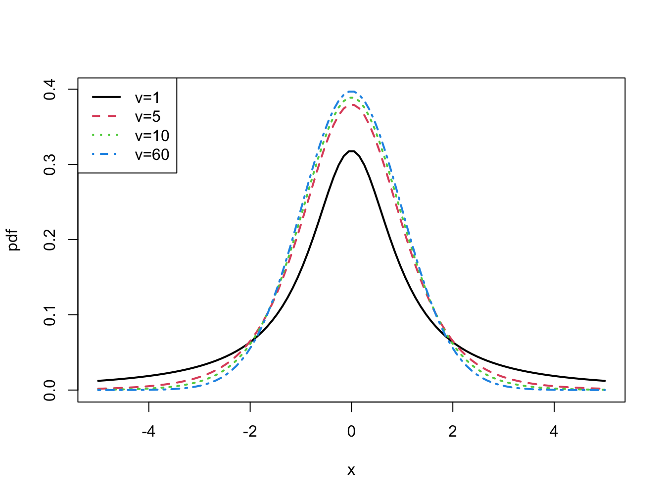
Figure 2.10: Student’s t density with \(v=1,5,10\) and \(60\).
The R functions pt() and qt() can be used to compute
the cdf and quantiles of a Student’s t random variable. For \(v=1,2,5,10,60,100\)
and \(\infty\) the 1% quantiles can be computed using:
## [1] -31.821 -6.965 -3.365 -2.764 -2.390 -2.364 -2.326For \(v=1,2,5,10,60,100\) and \(\infty\) the values of \(\Pr(X<-3)\) are:
## [1] 0.102416 0.047733 0.015050 0.006672 0.001964 0.001704 0.001350\(\blacksquare\)
2.1.7 Linear functions of a random variable
Let \(X\) be a random variable either discrete or continuous with \(E[X]=\mu_{X}\), \(\mathrm{var}(X)=\sigma_{X}^{2}\), and let \(a\) and \(b\) be known constants. Define a new random variable \(Y\) via the linear function of \(X\): \[ Y=g(X)=aX+b. \] Then the following results hold: \[\begin{align*} \mu_{Y} & =E[Y]=a\cdot E[X]+b=a\cdot\mu_{X}+b,\\ \sigma_{Y}^{2} & =\mathrm{var}(Y)=a^{2}\mathrm{var}(X)=a^{2}\sigma_{X}^{2},\\ \sigma_{Y} & =\mathrm{sd}(Y)=a\cdot\mathrm{sd}(X)=a\cdot\sigma_{X}. \end{align*}\] The first result shows that expectation is a linear operation. That is, \[ E[aX+b]=aE[X]+b. \] The second result shows that adding a constant to \(X\) does not affect its variance, and that the effect of multiplying \(X\) by the constant \(a\) increases the variance of \(X\) by the square of \(a.\) These results will be used often enough that it is instructive to go through the derivations.
Consider the first result. Let \(X\) be a discrete random variable. By the definition of \(E[g(X)]\), with \(g(X)=b+aX\), we have: \[\begin{align*} E[Y] & =\sum_{x\in S_{X}}(ax+b)\cdot\Pr(X=x)\\ & =a\sum_{x\in S_{X}}x\cdot\Pr(X=x)+b\sum_{x\in S_{X}}\Pr(X=x)\\ & =a\cdot E[X]+b\cdot1\\ & =a\cdot\mu_{X}+b. \end{align*}\] If \(X\) is a continuous random variable then by the linearity of integration: \[\begin{align*} E[Y] & =\int_{-\infty}^{\infty}(ax+b)f(x)~dx=a\int_{-\infty}^{\infty}xf(x)~dx+b\int_{-\infty}^{\infty}f(x)~dx\\ & =aE[X]+b. \end{align*}\] Next consider the second result. Since \(\mu_{Y}=a\mu_{X}+b\) we have: \[\begin{align*} \mathrm{var}(Y) & =E[(Y-\mu_{Y})^{2}]\\ & =E[(aX+b-(a\mu_{X}+b))^{2}]\\ & =E[(a(X-\mu_{X})+(b-b))^{2}]\\ & =E[a^{2}(X-\mu_{X})^{2}]\\ & =a^{2}E[(X-\mu_{X})^{2}]\textrm{ (by the linearity of }E[\cdot]\textrm{)}\\ & =a^{2}\mathrm{var}(X) \end{align*}\] Notice that the derivation of the second result works for discrete and continuous random variables.
A normal random variable has the special property that a linear function of it is also a normal random variable. The following proposition states the result.
Proposition 2.1 Let \(X\sim N(\mu_{X},\sigma_{X}^{2})\) and let \(a\) and \(b\) be constants. Let \(Y=aX+b\). Then \(Y\sim N(a\mu_{X}+b,a^{2}\sigma_{X}^{2})\).
The above property is special to the normal distribution and may or may not hold for a random variable with a distribution that is not normal.
Let \(X\) be a random variable with \(E[X]=\mu_{X}\) and \(\mathrm{var}(X)=\sigma_{X}^{2}\). Define a new random variable \(Z\) as: \[ Z=\frac{X-\mu_{X}}{\sigma_{X}}=\frac{1}{\sigma_{X}}X-\frac{\mu_{X}}{\sigma_{X}}, \] which is a linear function \(aX+b\) where \(a=\frac{1}{\sigma_{X}}\) and \(b=-\frac{\mu_{X}}{\sigma_{X}}\). This transformation is called standardizing the random variable \(X\) since, \[\begin{align*} E[Z] & =\frac{1}{\sigma_{X}}E[X]-\frac{\mu_{X}}{\sigma_{X}}=\frac{1}{\sigma_{X}}\mu_{X}-\frac{\mu_{X}}{\sigma_{X}}=0,\\ \mathrm{var}(Z) & =\left(\frac{1}{\sigma_{X}}\right)^{2}\mathrm{var}(X)=\frac{\sigma_{X}^{2}}{\sigma_{X}^{2}}=1. \end{align*}\] Hence, standardization creates a new random variable with mean zero and variance 1. In addition, if \(X\) is normally distributed then \(Z\sim N(0,1)\).
\(\blacksquare\)
Let \(X\sim N(2,4)\) and suppose we want to find \(\Pr(X>5)\) but we only know probabilities associated with a standard normal random variable \(Z\sim N(0,1)\). We solve the problem by standardizing \(X\) as follows: \[ \Pr\left(X>5\right)=\Pr\left(\frac{X-2}{\sqrt{4}}>\frac{5-2}{\sqrt{4}}\right)=\Pr\left(Z>\frac{3}{2}\right)=0.06681. \]
\(\blacksquare\)
Standardizing a random variable is often done in the construction of test statistics. For example, the so-called t-statistic or t-ratio used for testing simple hypotheses on coefficients is constructed by the standardization process.
A non-standard random variable \(X\) with mean \(\mu_{X}\) and variance \(\sigma_{X}^{2}\) can be created from a standard random variable via the linear transformation: \[\begin{equation} X=\mu_{X}+\sigma_{X}\cdot Z.\tag{2.23} \end{equation}\] This result is useful for modeling purposes as illustrated in the next examples.
Let \(X\sim N(\mu_{X},\sigma_{X}^{2})\). Quantiles of \(X\) can be conveniently computed using: \[\begin{equation} q_{\alpha}=\mu_{X}+\sigma_{X}z_{\alpha},\tag{2.24} \end{equation}\] where \(\alpha\in(0,1)\) and \(z_{\alpha}\) is the \(\alpha\times100\%\) quantile of a standard normal random variable. This formula is derived as follows. By the definition \(z_{\alpha}\) and (2.23) \[ \alpha=\Pr(Z\leq z_{\alpha})=\Pr\left(\mu_{X}+\sigma_{X}\cdot Z\leq\mu_{X}+\sigma_{X}\cdot z_{\alpha}\right)=\Pr(X\leq\mu_{X}+\sigma_{X}\cdot z_{\alpha}), \] which implies (2.24).
\(\blacksquare\)
The Student’s t distribution defined in (2.22) has zero mean and variance equal to \(v/(v-2)\) where \(v\) is the degrees of freedom parameter. We can define a Student’s t random variable with non-zero mean \(\mu\) and variance \(\sigma^{2}\) from a Student’s t random variable \(X\) as follows: \[ Y=\mu+\sigma\left(\frac{v-2}{v}\right)^{1/2}X=\mu+\sigma Z_{v}, \] where \(Z_{v}=\left(\frac{v-2}{v}\right)^{1/2}X\). The random variable \(Z_{v}\) is called a standardized Student’s t random variable with \(v\) degrees of freedom since \(E[Z_{v}]=0\) and \(\mathrm{var}(Z_{v})=\left(\frac{v-2}{v}\right)\mathrm{var}(X)=\left(\frac{v-2}{v}\right)\left(\frac{v}{v-2}\right)=1\). Then \[\begin{eqnarray*} E[Y] & = & \mu+\sigma E[Z]=\mu,\\ \mathrm{var}(Y) & = & \sigma^{2}\mathrm{var}(Z)=\sigma^{2}. \end{eqnarray*}\]
We use the notation \(Y \sim t_{v}(\mu, \sigma^{2})\) to denote that \(Y\) has a generalized Student’s t distribution with mean \(\mu\), variance \(\sigma^{2}\), and degrees of freedom \(v\).
\(\blacksquare\)
Let \(r\) denote the monthly continuously compounded return on an asset with \(E[r]=\mu\) and \(\mathrm{var}(R)=\sigma^{2}\). If \(r\) has a normal distribution or a general Student’s t distribution, then \(r\) can be expressed as: \[ r=\mu_{r}+\sigma_{r}\cdot\varepsilon, \] where \(\varepsilon \sim N(0,1)\) or \(\varepsilon \sim t_{v}(0,1)\). The random variable \(\varepsilon\) can be interpreted as representing the random news arriving in a given month that makes the observed return differ from its expected value \(\mu\). The fact that \(\varepsilon\) has mean zero means that news, on average, is neutral. The value of \(\sigma_{r}\) represents the typical size of a news shock. The bigger is \(\sigma_{r}\), the larger is the impact of a news shock and vice-versa. The distribution of \(\varepsilon\) impacts the likelihood of extreme new events (like stock market crashes). If \(\varepsilon \sim N(0,1)\) then extreme news events are not very likely. If \(\varepsilon \sim t_{v}(0,1)\) with \(v\) small (but bigger than 4) then extreme news events may happen from time-to-time.
\(\blacksquare\)
2.1.8 Value-at-Risk: An introduction
As an example of working with linear functions of a normal random variable, and to illustrate the concept of Value-at-Risk (VaR), consider an investment of $10,000 in Microsoft stock over the next month. Let \(R\) denote the monthly simple return on Microsoft stock and assume that \(R\sim N(0.05,(0.10)^{2})\). That is, \(E[R]=\mu_{R}=0.05\) and \(\mathrm{var}(R)=\sigma_{R}^{2}=(0.10)^{2}\). Let \(W_{0}\) denote the investment value at the beginning of the month and \(W_{1}\) denote the investment value at the end of the month. In this example, \(W_{0}=\$10,000\). Consider the following questions:
- What is the probability distribution of end-of-month wealth, \(W_{1}?\)
- What is the probability that end-of-month wealth is less than $9,000, and what must the return on Microsoft be for this to happen?
- What is the loss in dollars that would occur if the return on Microsoft stock is equal to its 5% quantile, \(q_{.05}\)? That is, what is the monthly 5% VaR on the $10,000 investment in Microsoft?
To answer (i), note that end-of-month wealth, \(W_{1}\), is related to initial wealth \(W_{0}\) and the return on Microsoft stock \(R\) via the linear function: \[ W_{1}=W_{0}(1+R)=W_{0}+W_{0}R=\$10,000+\$10,000\cdot R. \] Using the properties of linear functions of a random variable we have: \[ E[W_{1}]=W_{0}+W_{0}E[R]=\$10,000+\$10,000(0.05)=\$10,500, \] and, \[\begin{align*} \mathrm{var}(W_{1}) & =(W_{0})^{2}\mathrm{var}(R)=(\$10,000)^{2}(0.10)^{2},\\ \mathrm{sd}(W_{1}) & =(\$10,000)(0.10)=\$1,000. \end{align*}\] Further, since \(R\) is assumed to be normally distributed it follows that \(W_{1}\) is normally distributed: \[ W_{1}\sim N(\$10,500,(\$1,000)^{2}). \] To answer (ii), we use the above normal distribution for \(W_{1}\) to get: \[ \Pr(W_{1}<\$9,000)=0.067. \] To find the return that produces end-of-month wealth of $9,000, or a loss of $10,000-$9,000=$1,000, we solve \[ R=\frac{\$9,000-\$10,000}{\$10,000}=-0.10. \] If the monthly return on Microsoft is -10% or less, then end-of-month wealth will be $9,000 or less. Notice that \(R=-0.10\) is the 6.7% quantile of the distribution of \(R\): \[ \Pr(R<-0.10)=0.067. \] Question (iii) can be answered in two equivalent ways. First, we use \(R\sim N(0.05,(0.10)^{2})\) and solve for the 5% quantile of Microsoft Stock using (2.24)12: \[\begin{align*} \Pr(R & <q_{.05}^{R})=0.05\\ & \Rightarrow q_{.05}^{R}=\mu_{R}+\sigma_{R}\cdot z_{.05}=0.05+0.10\cdot(-1.645)=-0.114. \end{align*}\] That is, with 5% probability the return on Microsoft stock is -11.4% or less. Now, if the return on Microsoft stock is -11.4% the loss in investment value that occurs with 5% probability is \[ \mathrm{VaR}_{0.05} = W_{0}\cdot q_{.05}^{R} = \$10,000\cdot(0.114)= -\$1,144. \] Since losses are typically reported as positive numbers, \(\mathrm{VaR}_{0.05} = \$1,144\) is the 5% VaR over the next month on the $10,000 investment in Microsoft stock.
For the second method, use \(W_{1}\) ~ \(N(\$10,500,(\$1,000)^{2})\) and solve for the \(5\%\) quantile of end-of-month wealth directly: \[ \Pr(W_{1}<q_{.05}^{W_{1}})=0.05\Rightarrow q_{.05}^{W_{1}}=\$8,856. \] This corresponds to a loss of investment value of $10,000-$8,856=$1,144. Hence, if \(W_{0}\) represents the initial wealth and \(q_{.05}^{W_{1}}\) is the 5% quantile of the distribution of \(W_{1}\) then the 5% VaR is: \[ \textrm{ VaR}_{.05}=W_{0}-q_{.05}^{W_{1}}=\$10,000-\$8,856=\$1,144. \]
The following is the usual definition of VaR.Definition 2.14 If \(W_{0}\) represents the initial wealth in dollars and \(q_{\alpha}^{R}\) is the \(\alpha\times100\%\) quantile of distribution of the simple return \(R\) for small values of \(\alpha\), then the \(\alpha\times100\)% VaR is defined as: \[\begin{equation} \mathrm{VaR}_{\alpha}=-W_{0}\cdot q_{\alpha}^{R}.\tag{2.25} \end{equation}\]
In words, VaR\(_{\alpha}\) represents the dollar loss that could occur with probability \(\alpha\). By convention, it is reported as a positive number (hence the multiplication by minus one as \(q_{\alpha}^{R} < 0\) for small values of \(\alpha\)).
2.1.8.1 Value-at-Risk calculations for continuously compounded returns
The above calculations illustrate how to calculate VaR using the normal distribution for simple returns. However, as argued in Example 31, the normal distribution may not be appropriate for characterizing the distribution of simple returns and may be more appropriate for characterizing the distribution of continuously compounded returns. Let \(R\) denote the simple monthly return, let \(r=\ln(1+R)\) denote the continuously compounded return and assume that \(r\sim N(\mu_{r},\sigma_{r}^{2})\). The \(\alpha\times100\%\) monthly VaR on an investment of $\(W_{0}\) is computed using the following steps:
- Compute the \(\alpha\cdot100\%\) quantile, \(q_{\alpha}^{r}\), from the normal distribution for the continuously compounded return \(r\): \[ q_{\alpha}^{r}=\mu_{r}+\sigma_{r}z_{\alpha}, \] where \(z_{\alpha}\) is the \(\alpha\cdot100\%\) quantile of the standard normal distribution.
- Convert the continuously compounded return quantile, \(q_{\alpha}^{r}\), to a simple return quantile using the transformation: \[ q_{\alpha}^{R}=e^{q_{\alpha}^{r}}-1 \]
- Compute VaR using the simple return quantile (2.25).
Step 2 works because quantiles are preserved under monotonically increasing transformations of random variables.
Let \(R\) denote the simple monthly return on Microsoft stock and assume that \(R\sim N(0.05,(0.10)^{2})\). Consider an initial investment of \(W_{0}=\$10,000\). To compute the 1% and 5% VaR values over the next month use:
mu.R = 0.05
sd.R = 0.10
w0 = 10000
q.01.R = mu.R + sd.R*qnorm(0.01)
q.05.R = mu.R + sd.R*qnorm(0.05)
VaR.01 = -q.01.R*w0
VaR.05 = -q.05.R*w0
VaR.01
## [1] 1826## [1] 1145Hence with 1% and 5% probability the loss over the next month is at least $1,826 and $1,145, respectively.
Let \(r\) denote the continuously compounded return on Microsoft stock and assume that \(r\sim N(0.05,(0.10)^{2})\). To compute the 1% and 5% VaR values over the next month use:
mu.r = 0.05
sd.r = 0.10
q.01.R = exp(mu.r + sd.r*qnorm(0.01)) - 1
q.05.R = exp(mu.r + sd.r*qnorm(0.05)) - 1
VaR.01 = -q.01.R*w0
VaR.05 = -q.05.R*w0
VaR.01
## [1] 1669## [1] 1082Notice that when \(1+R=e^{r}\) has a log-normal distribution, the 1% and 5% VaR values (losses) are slightly smaller than when \(R\) is normally distributed. This is due to the positive skewness of the log-normal distribution.
\(\blacksquare\)
2.2 Bivariate Distributions
So far we have only considered probability distributions for a single random variable. In many situations, we want to be able to characterize the probabilistic behavior of two or more random variables simultaneously. For example, we might want to know about the probabilistic behavior of the returns on a two asset portfolio. In this section, we discuss bivariate distributions and important concepts related to the analysis of two random variables.
2.2.1 Discrete random variables
Let \(X\) and \(Y\) be discrete random variables with sample spaces \(S_{X}\) and \(S_{Y}\), respectively. The likelihood that \(X\) and \(Y\) takes values in the joint sample space \(S_{XY}=S_{X}\times S_{Y}\) (Cartesian product of the individual sample spaces) is determined by the joint probability distribution \(p(x,y)=\Pr(X=x,Y=y).\) The function \(p(x,y)\) satisfies:
- \(p(x,y)>0\) for \(x,y\in S_{XY}\);
- \(p(x,y)=0\) for \(x,y\notin S_{XY}\);
- \(\sum_{x,y\in S_{XY}}p(x,y)=\sum_{x\in S_{X}}\sum_{y\in S_{Y}}p(x,y)=1\).
Let \(X\) denote the monthly return (in percent) on Microsoft stock and let \(Y\) denote the monthly return on Starbucks stock. For simplicity suppose that the sample spaces for \(X\) and \(Y\) are \(S_{X}=\{0,1,2,3\}\) and \(S_{Y}=\{0,1\}\) so that the random variables \(X\) and \(Y\) are discrete. The joint sample space is the two dimensional grid \(S_{XY}=\{(0,0)\), \((0,1)\), \((1,0)\), \((1,1)\), \((2,0)\), \((2,1)\), \((3,0)\), \((3,1)\}\). Table 2.3 illustrates the joint distribution for \(X\) and \(Y\). From the table, \(p(0,0)=\Pr(X=0,Y=0)=1/8\). Notice that the sum of all the entries in the table sum to unity.
\(\blacksquare\)
+——+————–+———+———+————–+ | | |Y | | | +======+==============+=========+=========+==============+ | |% |0 |1 |\(\Pr(X)\) | +——+————–+———+———+————–+ | |0 |1/8 |0 |1/8 | +——+————–+———+———+————–+ |X |1 |2/8 |1/8 |3/8 | +——+————–+———+———+————–+ | |2 |1/8 |2/8 |3/8 | +——+————–+———+———+————–+ | |3 |0 |1/8 |1/8 | +——+————–+———+———+————–+ | |\(\Pr(Y)\) |4/8 |4/8 |1 | +——+————–+———+———+————–+ Table: (#tab:Table-bivariateDistn) Discrete bivariate distribution for Microsoft and Starbucks stock prices.
2.2.1.1 Marginal Distributions
The joint probability distribution tells us the probability of \(X\) and \(Y\) occurring together. What if we only want to know about the probability of \(X\) occurring, or the probability of \(Y\) occurring?
Consider the joint distribution in Table 2.3. What is \(\Pr(X=0)\) regardless of the value of \(Y\)? Now \(X\) can occur if \(Y=0\) or if \(Y=1\) and since these two events are mutually exclusive we have that \[ \Pr(X=0)=\Pr(X=0,Y=0)+\Pr(X=0,Y=1)=0+1/8=1/8. \] Notice that this probability is equal to the horizontal (row) sum of the probabilities in the table at \(X=0\). We can find \(\Pr(Y=1)\) in a similar fashion: \[\begin{align*} \Pr(Y=1)&=\Pr(X=0,Y=1)+\Pr(X=1,Y=1)+\Pr(X=2,Y=1)+\Pr(X=3,Y=1)\\ &=0+1/8+2/8+1/8=4/8. \end{align*}\] This probability is the vertical (column) sum of the probabilities in the table at \(Y=1\).
\(\blacksquare\)
The marginal probabilities of \(X=x\) are given in the last column of Table 2.3, and the marginal probabilities of \(Y=y\) are given in the last row of Table 2.3. Notice that these probabilities sum to 1. For future reference we note that \(E[X]=3/2,\mathrm{var}(X)=3/4,E[Y]=1/2\), and \(\mathrm{var}(Y)=1/4\).
\(\blacksquare\)
2.2.1.2 Conditional Distributions
For random variables in Table 2.3, suppose we know that the random variable \(Y\) takes on the value \(Y=0\). How does this knowledge affect the likelihood that \(X\) takes on the values 0, 1, 2 or 3? For example, what is the probability that \(X=0\) given that we know \(Y=0\)? To find this probability, we use Bayes’ law and compute the conditional probability: \[ \Pr(X=0|Y=0)=\frac{\Pr(X=0,Y=0)}{\Pr(Y=0)}=\frac{1/8}{4/8}=1/4. \] The notation \(\Pr(X=0|Y=0)\) is read as “the probability that \(X=0\) given that \(Y=0\)” . Notice that \(\Pr(X=0|Y=0)=1/4>\Pr(X=0)=1/8\). Hence, knowledge that \(Y=0\) increases the likelihood that \(X=0\). Clearly, \(X\) depends on \(Y\).
Now suppose that we know that \(X=0\). How does this knowledge affect the probability that \(Y=0?\) To find out we compute: \[ \Pr(Y=0|X=0)=\frac{\Pr(X=0,Y=0)}{\Pr(X=0)}=\frac{1/8}{1/8}=1. \] Notice that \(\Pr(Y=0|X=0)=1>\Pr(Y=0)=1/2\). That is, knowledge that \(X=0\) makes it certain that \(Y=0\).
For the bivariate distribution in Table 2.3, the conditional probabilities along with marginal probabilities are summarized in Tables 2.4 and 2.5. Notice that the marginal distribution of \(X\) is centered at \(x=3/2\) whereas the conditional distribution of \(X|Y=0\) is centered at \(x=1\) and the conditional distribution of \(X|Y=1\) is centered at \(x=2\).
\(\blacksquare\)
+—+————+————–+————–+ |x |\(\Pr(X=x)\) |\(\Pr(X|Y=0)\) |\(\Pr(X|Y=1)\) | +===+============+==============+==============+ |0 |1/8 |2/8 |0 | +—+————+————–+————–+ |1 |3/8 |4/8 |2/8 | +—+————+————–+————–+ |2 |3/8 |4/8 |4/8 | +—+————+————–+————–+ |3 |1/8 |0 |2/8 | +—+————+————–+————–+ Table: (#tab:Table-ConditionalDistnX) Conditional probability distribution of X from bivariate discrete distribution.
+—+————+————–+————–+————–+————–+ |y |\(\Pr(Y=y)\) |\(\Pr(Y|X=0)\) |\(\Pr(Y|X=1)\) |\(\Pr(Y|X=2)\) |\(\Pr(Y|X=3)\) | +—+————+————–+————–+————–+————–+ |0 |1/2 |1 |2/3 |1/3 |0 | +—+————+————–+————–+————–+————–+ |1 |1/2 |0 |1/3 |2/3 |1 | +—+————+————–+————–+————–+————–+ Table: (#tab:Table-ConditionalDistnY) Conditional distribution of Y from bivariate discrete distribution.
2.2.1.3 Conditional expectation and conditional variance
Just as we defined shape characteristics of the marginal distributions of \(X\) and \(Y\), we can also define shape characteristics of the conditional distributions of \(X|Y=y\) and \(Y|X=x\). The most important shape characteristics are the conditional expectation (conditional mean) and the conditional variance. The conditional mean of \(X|Y=y\) is denoted by \(\mu_{X|Y=y}=E[X|Y=y]\), and the conditional mean of \(Y|X=x\) is denoted by \(\mu_{Y|X=x}=E[Y|X=x]\).Definition 2.17 For discrete random variables \(X\) and \(Y\), the conditional expectations are defined as: \[\begin{align} \mu_{X|Y=y} & =E[X|Y=y]=\sum_{x\in S_{X}}x\cdot\Pr(X=x|Y=y),\tag{2.30}\\ \mu_{Y|X=x} & =E[Y|X=x]=\sum_{y\in S_{Y}}y\cdot\Pr(Y=y|X=x).\tag{2.31} \end{align}\]
Definition 2.18 For discrete random variables \(X\) and \(Y\), the conditional variances are defined as: \[\begin{align} \sigma_{X|Y=y}^{2} & =\mathrm{var}(X|Y=y)=\sum_{x\in S_{X}}(x-\mu_{X|Y=y})^{2}\cdot\Pr(X=x|Y=y),\tag{2.32}\\ \sigma_{Y|X=x}^{2} & =\mathrm{var}(Y|X=x)=\sum_{y\in S_{Y}}(y-\mu_{Y|X=x})^{2}\cdot\Pr(Y=y|X=x).\tag{2.33} \end{align}\] The conditional volatilities are defined as: \[\begin{align} \sigma_{X|Y=y} & = \sqrt{\sigma_{X|Y=y}^{2}}, \tag{2.34}\\ \sigma_{Y|X=x} & = \sqrt{\sigma_{Y|X=x}^{2}}. \tag{2.35} \end{align}\]
Then conditional mean is the center of mass of the conditional distribution, and the conditional variance and volatility measure the spread of the conditional distribution about the conditional mean.
For the random variables in Table 2.3, we have the following conditional moments for \(X\): \[\begin{align*} E[X|Y & =0]=0\cdot1/4+1\cdot1/2+2\cdot1/4+3\cdot0=1,\\ E[X|Y & =1]=0\cdot0+1\cdot1/4+2\cdot1/2+3\cdot1/4=2,\\ \mathrm{var}(X|Y & =0)=(0-1)^{2}\cdot1/4+(1-1)^{2}\cdot1/2+(2-1)^{2}\cdot1/2+(3-1)^{2}\cdot0=1/2,\\ \mathrm{var}(X|Y & =1)=(0-2)^{2}\cdot0+(1-2)^{2}\cdot1/4+(2-2)^{2}\cdot1/2+(3-2)^{2}\cdot1/4=1/2. \end{align*}\] Compare these values to \(E[X]=3/2\) and \(\mathrm{var}(X)=3/4\). Notice that \(\mathrm{var}(X|Y) = 1/2 < \mathrm{var}(X)=3/4\) so that conditioning on information reduces variability. Also, notice that as \(y\) increases, \(E[X|Y=y]\) increases.
For \(Y\), similar calculations gives: \[\begin{align*} E[Y|X & =0]=0,E[Y|X=1]=1/3,E[Y|X=2]=2/3,E[Y|X=3]=1,\\ \mathrm{var}(Y|X & =0)=0,\mathrm{var}(Y|X=1)=0.2222,\mathrm{var}(Y|X=2)=0.2222,\mathrm{var}(Y|X=3)=0. \end{align*}\] Compare these values to \(E[Y]=1/2\) and \(\mathrm{var}(Y)=1/4\). Notice that as \(x\) increases \(E[Y|X=x]\) increases.
\(\blacksquare\)
2.2.1.4 Conditional expectation and the regression function
Consider the problem of predicting the value \(Y\) given that we know \(X=x\). A natural predictor to use is the conditional expectation \(E[Y|X=x]\). In this prediction context, the conditional expectation \(E[Y|X=x]\) is called the regression function. The graph with \(E[Y|X=x]\) on the vertical axis and \(x\) on the horizontal axis gives the regression line. The relationship between \(Y\) and the regression function may be expressed using the trivial identity: \[\begin{align} Y & =E[Y|X=x]+Y-E[Y|X=x]\nonumber \\ & =E[Y|X=x]+\varepsilon,\tag{2.36} \end{align}\] where \(\varepsilon=Y-E[Y|X]\) is called the regression error.
For the random variables in Table 2.3, the regression line is plotted in Figure 2.11. Notice that there is a linear relationship between \(E[Y|X=x]\) and \(x\). When such a linear relationship exists we call the regression function a linear regression. Linearity of the regression function, however, is not guaranteed. It may be the case that there is a non-linear (e.g., quadratic) relationship between \(E[Y|X=x]\) and \(x\). In this case, we call the regression function a non-linear regression.
\(\blacksquare\)
![Regression function $E[Y|X=x]$ from discrete bivariate distribution.](_main_files/figure-html/figProbReviewDiscreteRegression-1.png)
Figure 2.11: Regression function \(E[Y|X=x]\) from discrete bivariate distribution.
2.2.1.5 Law of Total Expectations
Before \(Y\) is observed, \(E[X|Y]\) is a random variable because its value depends on the value of \(Y\) which is a random variable. Similarly, \(E[Y|X]\) is also a random variable. Since \(E[X|Y]\) and \(E[Y|X]\) are random variables we can consider their mean values. To illustrate, for the random variables in Table 2.3 notice that: \[\begin{align*} E[X] & = sum_{y \in S_{Y}} E[X|Y=y]\cdot \Pr(Y=y)\\ & =E[X|Y=0]\cdot\Pr(Y=0)+E[X|Y=1]\cdot\Pr(Y=1)\\ & =1\cdot1/2+2\cdot1/2=3/2, \end{align*}\] and, \[\begin{align*} E[Y] & = sum_{x \in S_{X}} E[Y|X=x]\cdot \Pr(X=x)\\ & =E[Y|X=0]\cdot\Pr(X=0)+E[Y|X=1]\cdot\Pr(X=1)\\ +E[Y|X & =2]\cdot\Pr(X=2)+E[Y|X=3]\cdot\Pr(X=3)=1/2. \end{align*}\] This result is known as the law of total expectations.In words, the law of total expectations says that the mean of the conditional mean is the unconditional mean.
2.2.2 Bivariate distributions for continuous random variables
Let \(X\) and \(Y\) be continuous random variables defined over the real line. We characterize the joint probability distribution of \(X\) and \(Y\) using the joint probability function (pdf) \(f(x,y)\) such that \(f(x,y)\geq0\) and, \[ \int_{-\infty}^{\infty}\int_{-\infty}^{\infty}f(x,y)~dx~dy=1. \] The three-dimensional plot of the joint probability distribution gives a probability surface whose total volume is unity. To compute joint probabilities of \(x_{1}\leq X\leq x_{2}\) and \(y_{1}\leq Y\leq y_{2},\) we need to find the volume under the probability surface over the grid where the intervals \([x_{1},x_{2}]\) and \([y_{1},y_{2}]\) overlap. Finding this volume requries solving the double integral: \[ \Pr(x_{1}\leq X\leq x_{2},y_{1}\leq Y\leq y_{2})=\int_{x_{1}}^{x_{2}}\int_{y_{1}}^{y_{2}}f(x,y)~dx~dy. \]
A standard bivariate normal pdf for \(X\) and \(Y\) has the form:
\[\begin{equation}
f(x,y)=\frac{1}{2\pi}e^{-\frac{1}{2}(x^{2}+y^{2})},~-\infty\leq x,~y\leq\infty\tag{2.38}
\end{equation}\]
and has the shape of a symmetric bell (think Liberty Bell) centered
at \(x=0\) and \(y=0\). To find \(\Pr(-1<X<1,-1<Y<1)\) we must solve:
\[
\int_{-1}^{1}\int_{-1}^{1}\frac{1}{2\pi}e^{-\frac{1}{2}(x^{2}+y^{2})}~dx~dy,
\]
which, unfortunately, does not have an analytical solution. Numerical
approximation methods are required to evaluate the above integral.
The function pmvnorm() in the R package mvtnorm can be used
to evaluate areas under the bivariate standard normal surface. To
compute \(\Pr(-1<X<1,-1<Y<1)\) use:
## [1] 0.4661
## attr(,"error")
## [1] 1e-15
## attr(,"msg")
## [1] "Normal Completion"
Here, \(\Pr(-1<X<1,-1<Y<1)=0.4661\). The attribute error gives
the estimated absolute error of the approximation, and the attribute
message tells the status of the algorithm used for the approximation.
See the online help for pmvnorm for more details.
\(\blacksquare\)
2.2.2.1 Marginal and conditional distributions
The marginal pdf of \(X\) is found by integrating \(y\) out of the joint pdf \(f(x,y)\) and the marginal pdf of \(Y\) is found by integrating \(x\) out of the joint pdf \(f(x,y)\): \[\begin{align} f(x) & =\int_{-\infty}^{\infty}f(x,y)~dy,\tag{2.39}\\ f(y) & =\int_{-\infty}^{\infty}f(x,y)~dx.\tag{2.40} \end{align}\] The conditional pdf of \(X\) given that \(Y=y\), denoted \(f(x|y)\), is computed as \[\begin{equation} f(x|y)=\frac{f(x,y)}{f(y)},\tag{2.41} \end{equation}\] and the conditional pdf of \(Y\) given that \(X=x\) is computed as, \[\begin{equation} f(y|x)=\frac{f(x,y)}{f(x)}.\tag{2.42} \end{equation}\] The conditional means are computed as \[\begin{align} \mu_{X|Y=y} & =E[X|Y=y]=\int x\cdot p(x|y)~dx,\tag{2.43}\\ \mu_{Y|X=x} & =E[Y|X=x]=\int y\cdot p(y|x)~dy,\tag{2.44} \end{align}\] and the conditional variances are computed as, \[\begin{align} \sigma_{X|Y=y}^{2} & =\mathrm{var}(X|Y=y)=\int(x-\mu_{X|Y=y})^{2}p(x|y)~dx,\tag{2.45}\\ \sigma_{Y|X=x}^{2} & =\mathrm{var}(Y|X=x)=\int(y-\mu_{Y|X=x})^{2}p(y|x)~dy.\tag{2.46} \end{align}\]
Suppose \(X\) and \(Y\) are distributed bivariate standard normal. To find the marginal distribution of \(X\) we use (2.39) and solve: \[ f(x)=\int_{-\infty}^{\infty}\frac{1}{2\pi}e^{-\frac{1}{2}(x^{2}+y^{2})}~dy=\frac{1}{\sqrt{2\pi}}e^{-\frac{1}{2}x^{2}}\int_{-\infty}^{\infty}\frac{1}{\sqrt{2\pi}}e^{-\frac{1}{2}y^{2}}~dy=\frac{1}{\sqrt{2\pi}}e^{-\frac{1}{2}x^{2}}. \] Hence, the marginal distribution of \(X\) is standard normal. Similiar calculations show that the marginal distribution of \(Y\) is also standard normal. To find the conditional distribution of \(X|Y=y\) we use (2.41) and solve: \[\begin{align*} f(x|y) & =\frac{f(x,y)}{f(x)}=\frac{\frac{1}{2\pi}e^{-\frac{1}{2}(x^{2}+y^{2})}}{\frac{1}{\sqrt{2\pi}}e^{-\frac{1}{2}y^{2}}}\\ & =\frac{1}{\sqrt{2\pi}}e^{-\frac{1}{2}(x^{2}+y^{2})+\frac{1}{2}y^{2}}\\ & =\frac{1}{\sqrt{2\pi}}e^{-\frac{1}{2}x^{2}}\\ & =f(x) \end{align*}\] So, for the standard bivariate normal distribution \(f(x|y)=f(x)\) which does not depend on \(y\). Similar calculations show that \(f(y|x)=f(y)\).
\(\blacksquare\)
2.2.3 Independence
Let \(X\) and \(Y\) be two discrete random variables. Intuitively, \(X\) is independent of \(Y\) if knowledge about \(Y\) does not influence the likelihood that \(X=x\) for all possible values of \(x\in S_{X}\) and \(y\in S_{Y}\). Similarly, \(Y\) is independent of \(X\) if knowledge about \(X\) does not influence the likelihood that \(Y=y\) for all values of \(y\in S_{Y}\). We represent this intuition formally for discrete random variables as follows.
For the data in Table 2.3, we know that \(\Pr(X=0|Y=0)=1/4\neq\Pr(X=0)=1/8\) so \(X\) and \(Y\) are not independent.
\(\blacksquare\)
Intuition for the above result follows from: \[\begin{align*} \Pr(X & =x|Y=y)&=\frac{\Pr(X=x,Y=y)}{\Pr(Y=y)}=\frac{\Pr(X=x)\cdot\Pr(Y=y)}{\Pr(Y=y)}\\ &=\Pr(X=x),\\ \Pr(Y & =y|X=x)&=\frac{\Pr(X=x,Y=y)}{\Pr(X=x)}=\frac{\Pr(X=x)\cdot\Pr(Y=y)}{\Pr(X=x)}\\ & =\Pr(Y=y), \end{align*}\] which shows that \(X\) and \(Y\) are independent.
For continuous random variables, we have the following definition of independence.
As with discrete random variables, we have the following result for continuous random variables.
This result is extremely useful in practice because it gives us an easy way to compute the joint pdf for two independent random variables: we simply compute the product of the marginal distributions.
Let \(X\sim N(0,1)\), \(Y\sim N(0,1)\) and let \(X\) and \(Y\) be independent. Then, \[ f(x,y)=f(x)f(y)=\frac{1}{\sqrt{2\pi}}e^{-\frac{1}{2}x^{2}}\frac{1}{\sqrt{2\pi}}e^{-\frac{1}{2}y^{2}}=\frac{1}{2\pi}e^{-\frac{1}{2}(x^{2}+y^{2})}. \] This result is a special case of the general bivariate normal distribution to be discussed in the next sub-section.
\(\blacksquare\)
A useful property of the independence between two random variables is the following Proposition.
For example, if \(X\) and \(Y\) are independent then \(X^{2}\) and \(Y^{2}\) are also independent.
2.2.4 Covariance and correlation
Let \(X\) and \(Y\) be two discrete random variables. Figure 2.12 displays several bivariate probability scatterplots (where equal probabilities are given on the dots). In panel (a) we see no linear relationship between \(X\) and \(Y\). In panel (b) we see a perfect positive linear relationship between \(X\) and \(Y\) and in panel (c) we see a perfect negative linear relationship. In panel (d) we see a positive, but not perfect, linear relationship; in panel (e) we see a negative, but not perfect, linear relationship. Finally, in panel (f) we see no systematic linear relationship but we see a strong nonlinear (parabolic) relationship. The covariance between \(X\) and \(Y\) measures the direction of the linear relationship between the two random variables. The correlation between \(X\) and \(Y\) measures the direction and the strength of the linear relationship between the two random variables.
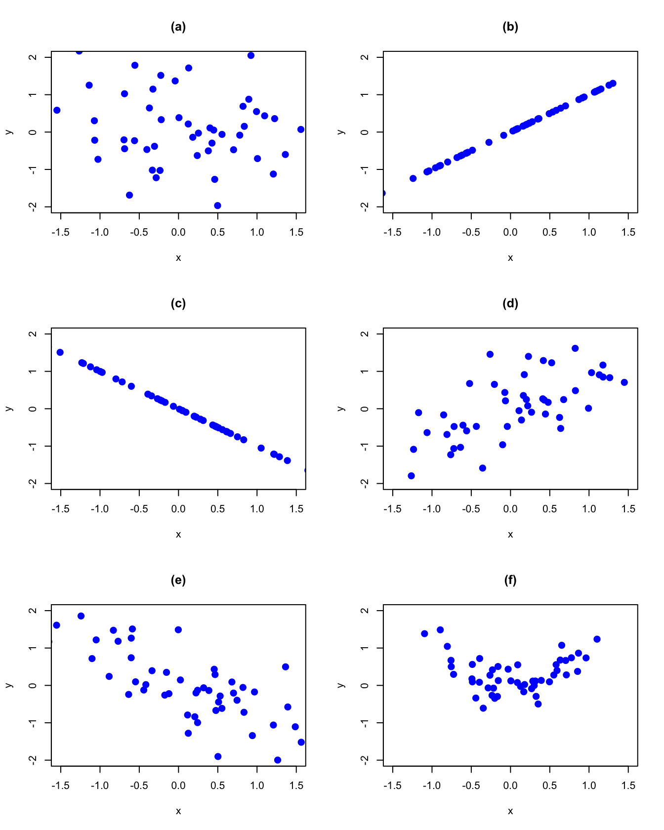
Figure 2.12: Probability scatterplots illustrating dependence between \(X\) and \(Y\).
Let \(X\) and \(Y\) be two random variables with \(E[X]=\mu_{X}\), \(\mathrm{var}(X)=\sigma_{X}^{2},E[Y]=\mu_{Y}\) and \(\mathrm{var}(Y)=\sigma_{Y}^{2}\).
To see how covariance measures the direction of linear association, consider the probability scatterplot in Figure 2.13. In the figure, each pair of points occurs with equal probability. The plot is separated into quadrants (right to left, top to bottom). In the first quadrant (black circles), the realized values satisfy \(x<\mu_{X},y>\mu_{Y}\) so that the product \((x-\mu_{X})(y-\mu_{Y})<0\). In the second quadrant (blue squares), the values satisfy \(x>\mu_{X}\) and \(y>\mu_{Y}\) so that the product \((x-\mu_{X})(y-\mu_{Y})>0\). In the third quadrant (red triangles), the values satisfy \(x<\mu_{X}\) and \(y<\mu_{Y}\) so that the product \((x-\mu_{X})(y-\mu_{Y})>0\). Finally, in the fourth quadrant (green diamonds), \(x>\mu_{X}\) but \(y<\mu_{Y}\) so that the product \((x-\mu_{X})(y-\mu_{Y})<0\). Covariance is then a probability weighted average all of the product terms in the four quadrants. For the values in Figure 2.13, this weighted average is positive because most of the values are in the second and third quadrants.
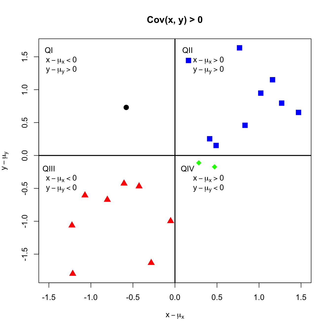
Figure 2.13: Probability scatterplot of discrete distribution with positive covariance. Each pair \((X,Y)\) occurs with equal probability.
For the data in Table 2.3, we have: \[\begin{gather*} \sigma_{XY}=\mathrm{cov}(X,Y)=(0-3/2)(0-1/2)\cdot1/8+(0-3/2)(1-1/2)\cdot0\\ +\cdots+(3-3/2)(1-1/2)\cdot1/8=1/4\\ \rho_{XY}=\mathrm{cor}(X,Y)=\frac{1/4}{\sqrt{(3/4)\cdot(1/2)}}=0.577 \end{gather*}\]
\(\blacksquare\)
2.2.4.1 Properties of covariance and correlation
Let \(X\) and \(Y\) be random variables and let \(a\) and \(b\) be constants. Some important properties of \(\mathrm{cov}(X,Y)\) are summarized in the following Proposition:
Proposition 2.6 1. \(\mathrm{cov}(X,X)=\mathrm{var}(X)\) 2. \(\mathrm{cov}(X,Y)=\mathrm{cov}(Y,X)\) 3. \(\mathrm{cov}(X,Y)=E[XY]-E[X]E[Y]=E[XY]-\mu_{X}\mu_{Y}\) 4. \(\mathrm{cov}(aX,bY)=a\cdot b\cdot\mathrm{cov}(X,Y)\) 5. If \(X\) and \(Y\) are independent then \(\mathrm{cov}(X,Y)=0\) (no association \(\Longrightarrow\) no linear association). However, if \(\mathrm{cov}(X,Y)=0\) then \(X\) and \(Y\) are not necessarily independent (no linear association \(\nRightarrow\) no association). 6. If \(X\) and \(Y\) are jointly normally distributed and \(\mathrm{cov}(X,Y)=0\), then \(X\) and \(Y\) are independent.
The first two properties are intuitive. The third property results from expanding the definition of covariance: \[\begin{align*} \mathrm{cov}(X,Y) & =E[(X-\mu_{X})(Y-\mu_{Y})]\\ & =E\left[XY-X\mu_{Y}-\mu_{X}Y+\mu_{X}\mu_{Y}\right]\\ & =E[XY]-E[X]\mu_{Y}-\mu_{X}E[Y]+\mu_{X}\mu_{Y}\\ & =E[XY]-2\mu_{X}\mu_{Y}+\mu_{X}\mu_{Y}\\ & =E[XY]-\mu_{X}\mu_{Y} \end{align*}\] The fourth property follows from the linearity of expectations: \[\begin{align*} \mathrm{cov}(aX,bY) & =E[(aX-a\mu_{X})(bY-b\mu_{Y})]\\ & =a\cdot b\cdot E[(X-\mu_{X})(Y-\mu_{Y})]\\ & =a\cdot b\cdot\mathrm{cov}(X,Y) \end{align*}\] The fourth property shows that the value of \(\mathrm{cov}(X,Y)\) depends on the scaling of the random variables \(X\) and \(Y\). By simply changing the scale of \(X\) or \(Y\) we can make \(\mathrm{cov}(X,Y)\) equal to any value that we want. Consequently, the numerical value of \(\mathrm{cov}(X,Y)\) is not informative about the strength of the linear association between \(X\) and \(Y\). However, the sign of \(\mathrm{cov}(X,Y)\) is informative about the direction of linear association between \(X\) and \(Y\).
The fifth property should be intuitive. Independence between the random variables \(X\) and \(Y\) means that there is no relationship, linear or nonlinear, between \(X\) and \(Y\). However, the lack of a linear relationship between \(X\) and \(Y\) does not preclude a nonlinear relationship.
The last result illustrates an important property of the normal distribution: lack of covariance implies independence.
Some important properties of \(\mathrm{cor}(X,Y)\) are:
TBD: discuss the results briefly
2.2.5 Bivariate normal distributions
Let \(X\) and \(Y\) be distributed bivariate normal. The joint pdf is given by: \[\begin{align} &f(x,y)=\frac{1}{2\pi\sigma_{X}\sigma_{Y}\sqrt{1-\rho_{XY}^{2}}}\times\tag{2.47}\\ &\exp\left\{ -\frac{1}{2(1-\rho_{XY}^{2})}\left[\left(\frac{x-\mu_{X}}{\sigma_{X}}\right)^{2}+\left(\frac{y-\mu_{Y}}{\sigma_{Y}}\right)^{2}-\frac{2\rho_{XY}(x-\mu_{X})(y-\mu_{Y})}{\sigma_{X}\sigma_{Y}}\right]\right\} \nonumber \end{align}\] where \(E[X]=\mu_{X}\), \(E[Y]=\mu_{Y}\), \(\mathrm{sd}(X)=\sigma_{X}\), \(\mathrm{sd}(Y)=\sigma_{Y}\), and \(\rho_{XY}=\mathrm{cor}(X,Y)\). The correlation coefficient \(\rho_{XY}\) describes the dependence between \(X\) and \(Y\). If \(\rho_{XY}=0\) then the pdf collapses to the pdf of the standard bivariate normal distribution. In this case, \(X\) and \(Y\) are independent random variables since \(f(x,y)=f(x)f(y).\)
It can be shown that the marginal distributions of \(X\) and \(Y\) are normal: \(X\sim N(\mu_{X},\sigma_{X}^{2})\), \(Y\sim N(\mu_{Y},\sigma_{Y}^{2})\). In addition, it can be shown that the conditional distributions \(f(x|y)\) and \(f(y|x)\) are also normal with means given by: \[\begin{align} \mu_{X|Y=y} & =\alpha_{X}+\beta_{X}\cdot y,\tag{2.48}\\ \mu_{Y|X=x} & =\alpha_{Y}+\beta_{Y}\cdot x,\tag{2.49} \end{align}\] where, \[\begin{align*} \alpha_{X} & =\mu_{X}-\beta_{X}\mu_{X},~\beta_{X}=\sigma_{XY}/\sigma_{Y}^{2},\\ \alpha_{Y} & =\mu_{Y}-\beta_{Y}\mu_{X},~\beta_{Y}=\sigma_{XY}/\sigma_{X}^{2}, \end{align*}\] and variances given by, \[\begin{align*} \sigma_{X|Y=y}^{2} & =\sigma_{X}^{2}-\sigma_{XY}^{2}/\sigma_{Y}^{2},\\ \sigma_{X|Y=y}^{2} & =\sigma_{Y}^{2}-\sigma_{XY}^{2}/\sigma_{X}^{2}. \end{align*}\] Notice that the conditional means (regression functions) (2.43) and (2.44) are linear functions of \(x\) and \(y\), respectively.
The formula for the bivariate normal distribution (2.47) is a bit messy. We can greatly simplify the formula by using matrix algebra. Define the \(2\times1\) vectors \(\mathbf{x}=(x,y)^{\prime}\) and \(\mu=(\mu_{X},\mu_{y})^{\prime},\) and the \(2\times2\) matrix: \[ \Sigma=\left(\begin{array}{cc} \sigma_{X}^{2} & \sigma_{XY}\\ \sigma_{XY} & \sigma_{Y}^{2} \end{array}\right) \] Then the bivariate normal distribution (2.47) may be compactly expressed as: \[\begin{equation} f(\mathbf{x})=\frac{1}{2\pi\det(\Sigma)^{1/2}}e^{-\frac{1}{2}(\mathbf{x}-\mu)^{\prime}\Sigma^{-1}(\mathbf{x}-\mu)} \tag{2.50} \end{equation}\] where, \[\begin{align*} \det(\Sigma)&=\sigma_{X}^{2}\sigma_{Y}^{2}-\sigma_{XY}^{2}=\sigma_{X}^{2}\sigma_{Y}^{2}-\sigma_{X}^{2}\sigma_{Y}^{2}\rho_{XY}^{2}=\sigma_{X}^{2}\sigma_{Y}^{2}(1-\rho_{XY}^{2})\\ \Sigma^{-1} &= \frac{1}{\det(\Sigma)} \left(\begin{array}{cc} \sigma_{Y}^{2} & -\sigma_{XY}\\ -\sigma_{XY} & \sigma_{X}^{2} \end{array}\right) \end{align*}\]
\(\blacksquare\)
The R package mvtnorm contains the functions dmvnorm(),
pmvnorm(), and qmvnorm() which can be used to compute
the bivariate normal pdf, cdf and quantiles, respectively. Plotting
the bivariate normal distribution over a specified grid of \(x\) and
\(y\) values in R can be done with the persp() function. First,
we specify the parameter values for the joint distribution. Here,
we choose \(\mu_{X}=\mu_{Y}=0\), \(\sigma_{X}=\sigma_{Y}=1\) and \(\rho=0.5\).
We will use the dmvnorm() function to evaluate the joint
pdf at these values. To do so, we must specify a covariance matrix
of the form:
\[
\Sigma=\left(\begin{array}{cc}
\sigma_{X}^{2} & \sigma_{XY}\\
\sigma_{XY} & \sigma_{Y}^{2}
\end{array}\right)=\left(\begin{array}{cc}
1 & 0.5\\
0.5 & 1
\end{array}\right).
\]
In R this matrix can be created using:
Next we specify a grid of \(x\) and \(y\) values between \(-3\) and \(3\):
To evaluate the joint pdf over the two-dimensional grid we can use
the outer() function:
# function to evaluate bivariate normal pdf on grid
bv.norm <- function(x, y, sigma) {
  z = cbind(x,y)
  return(dmvnorm(z, sigma=sigma))
}
# use outer function to evaluate pdf on 2D grid of x-y values
fxy = outer(x, y, bv.norm, sigma)
To create the 3D plot of the joint pdf, use the persp() function:
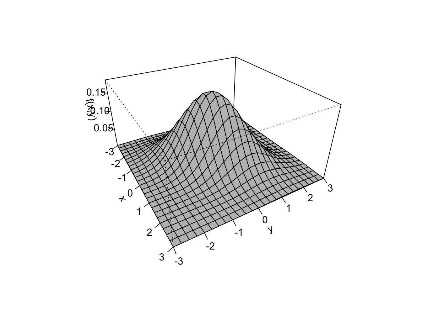
Figure 2.14: Bivariate normal pdf with \(\mu_{X}=\mu_{Y}=0\), \(\sigma_{X}\sigma_{Y}=1\) and \(\rho=0.5\).
The resulting plot is given in Figure 2.14.
\(\blacksquare\)
2.2.6 Expectation and variance of the sum of two random variables
Proposition 2.8 Let \(X\) and \(Y\) be two random variables with well defined means, variances and covariance and let \(a\) and \(b\) be constants. Then the following results hold: \[\begin{align} E[aX+bY] & =aE[X]+bE[Y]=a\mu_{X}+b\mu_{Y} \tag{2.51} \\ \mathrm{var}(aX+bY) & =a^{2}\mathrm{var}(X)+b^{2}\mathrm{var}(Y)+2\cdot a\cdot b\cdot\mathrm{cov}(X,Y)\\ & =a^{2}\sigma_{X}^{2}+b^{2}\sigma_{Y}^{2}+2\cdot a\cdot b\cdot\sigma_{XY} \tag{2.52} \end{align}\]
The first result (2.51) states that the expected value of a linear combination of two random variables is equal to a linear combination of the expected values of the random variables. This result indicates that the expectation operator is a linear operator. In other words, expectation is additive. The second result (2.52) states that variance of a linear combination of random variables is not a linear combination of the variances of the random variables. In particular, notice that covariance comes up as a term when computing the variance of the sum of two (not independent) random variables. Hence, the variance operator is not, in general, a linear operator. That is, variance, in general, is not additive.
It is instructive to go through the derivation of these results. Let \(X\) and \(Y\) be discrete random variables. Then, \[\begin{align*} E[aX+bY] & =\sum_{x\in S_{X}}\sum_{y\in S_{y}}(ax+by)\Pr (X=x,Y=y)\\ & =\sum_{x\in S_{X}}\sum_{y\in S_{y}}ax\Pr(X=x,Y=y)+\sum_{x\in S_{X}}\sum_{y\in S_{y}}bx\Pr(X=x,Y=y)\\ & =a\sum_{x\in S_{X}}x\sum_{y\in S_{y}}\Pr(X=x,Y=y)+b\sum_{y\in S_{y}}y\sum_{x\in S_{X}}\Pr(X=x,Y=y)\\ & =a\sum_{x\in S_{X}}x\Pr(X=x)+b\sum_{y\in S_{y}}y\Pr(Y=y)\\ & =aE[X]+bE[Y]=a\mu_{X}+b\mu_{Y}. \end{align*}\] The result for continuous random variables is similar. Effectively, the summations are replaced by integrals and the joint probabilities are replaced by the joint pdf.
Next, let \(X\) and \(Y\) be discrete or continuous random variables. Then, using the definition of variance we get: \[\begin{align*} \mathrm{var}(aX+bY) & =E[(aX+bY-E[aX+bY])^{2}]\\ & =E[(aX+bY-a\mu_{X}-b\mu_{Y})^{2}]\\ & =E[(a(X-\mu_{X})+b(Y-\mu_{Y}))^{2}]\\ & =a^{2}E[(X-\mu_{X})^{2}]+b^{2}E[(Y-\mu_{Y})^{2}]+2\cdot a\cdot b\cdot E[(X-\mu_{X})(Y-\mu_{Y})]\\ & =a^{2}\mathrm{var}(X)+b^{2}\mathrm{var}(Y)+2\cdot a\cdot b\cdot\mathrm{cov}(X,Y). \end{align*}\]
2.2.6.1 Linear combination of two normal random variables
The following proposition gives an important result concerning a linear combination of normal random variables.
This important result states that a linear combination of two normally distributed random variables is itself a normally distributed random variable. The proof of the result relies on the change of variables theorem from calculus and is omitted. Not all random variables have the nice property that their distributions are closed under addition.
Consider a portfolio of two stocks \(A\) (Amazon) and \(B\) (Boeing) with investment shares \(x_{A}\) and \(x_{B}\) with \(x_{A}+x_{B}=1\). Let \(R_{A}\) and \(R_{B}\) denote the simple monthly returns on these assets, and assume that \(R_{A}\sim N(\mu_{A},\sigma_{A}^{2})\) and \(R_{B}\sim N(\mu_{B},\sigma_{B}^{2})\). Furthermore, let \(\sigma_{AB}=\rho_{AB}\sigma_{A}\sigma_{B}=\mathrm{cov}(R_{A},R_{B})\). The portfolio return is \(R_{p}=x_{A}R_{A}+x_{B}R_{B}\), which is a linear function of two random variables. Using the properties of linear functions of random variables, we have: \[\begin{align*} \mu_{p} & =E[R_{p}]=x_{A}E[R_{A}]+x_{B}E[R_{B}]=x_{A}\mu_{A}+x_{B}\mu_{B}\\ \sigma_{p}^{2} & =\mathrm{var}(R_{p})=x_{A}^{2}\mathrm{var}(R_{A})+x_{B}^{2}\mathrm{var}(R_{B})+2x_{A}x_{B}\mathrm{cov}(R_{A},R_{B})\\ & =x_{A}^{2}\sigma_{A}^{2}+x_{B}^{2}\sigma_{B}^{2}+2x_{A}x_{B}\sigma_{AB}. \end{align*}\]
\(\blacksquare\)
2.3 Multivariate Distributions
Multivariate distributions are used to characterize the joint distribution of a collection of \(N\) random variables \(X_{1},X_{2},\ldots,X_{N}\) for \(N>1\). The mathematical formulation of this joint distribution can be quite complex and typically makes use of matrix algebra. Here, we summarize some basic properties of multivariate distributions without the use of matrix algebra. In chapter 3, we show how matrix algebra can greatly simplify the description of multivariate distributions.
2.3.1 Discrete random variables
Let \(X_{1},X_{2},\ldots,X_{N}\) be \(N\) discrete random variables with sample spaces \(S_{X_{1}},S_{X_{2}},\ldots,S_{X_{N}}\). The likelihood that these random variables take values in the joint sample space \(S_{X_{1}}\times S_{X_{2}}\times\cdots\times S_{X_{N}}\) is given by the joint probability function: \[ p(x_{1},x_{2},\ldots,x_{N})=\Pr(X_{1}=x_{1},X_{2}=x_{2},\ldots,X_{N}=x_{N}). \] For \(N>2\) it is not easy to represent the joint probabilities in a table like Table 2.3 or to visualize the distribution.
Marginal distributions for each variable \(X_{i}\) can be derived from the joint distribution as in (2.26) by summing the joint probabilities over the other variables \(j\neq i\). For example, \[ p(x_{1})=\sum_{x_{2}\in S_{X_{2}},\ldots,x_{N}\in S_{X_{N}}}p(x_{1},x_{2},\ldots,x_{N}). \] With \(N\) random variables, there are numerous conditional distributions that can be formed. For example, the distribution of \(X_{1}\) given \(X_{2}=x_{2},\ldots,X_{N}=x_{N}\) is determined using: \[ \Pr(X_{1}=x_{1}|X_{2}=x_{2},\ldots,X_{N}=x_{N})=\frac{\Pr(X_{1}=x_{1},X_{2}=x_{2},\ldots,X_{N}=x_{N})}{\Pr(X_{2}=x_{2},\ldots,X_{N}=x_{N})}. \] Similarly, the joint distribution of \(X_{1}\) and \(X_{2}\) given \(X_{3}=x_{3},\ldots,X_{N}=x_{N}\) is given by: \[\begin{align*} \Pr(X_{1}=x_{1},X_{2}=x_{2}|X_{3}=x_{3},\ldots,X_{N}=x_{N}) \\ =\frac{\Pr(X_{1}=x_{1},X_{2}=x_{2},\ldots,X_{N}=x_{N})}{\Pr(X_{3}=x_{3},\ldots,X_{N}=x_{N})}. \end{align*}\]
2.3.2 Continuous random variables
Let \(X_{1},X_{2},\ldots,X_{N}\) be \(N\) continuous random variables each taking values on the real line. The joint pdf is a function \(f(x_{1},x_{2},\ldots,x_{N})\geq0\) such that: \[ \int_{-\infty}^{\infty}\int_{-\infty}^{\infty}\cdots\int_{-\infty}^{\infty}f(x_{1},x_{2},\ldots,x_{N})~dx_{1}~dx_{2}\cdots~dx_{N}=1. \] Joint probabilities of \(x_{11}\leq X_{1}\leq x_{12},x_{21}\leq X_{2}\leq x_{22},\ldots,x_{N1}\leq X_{N}\leq x_{N2}\) are computed by solving the integral equation: \[\begin{equation} \int_{x_{11}}^{x_{12}}\int_{x_{21}}^{x_{22}}\cdots\int_{x_{N1}}^{x_{N2}}f(x_{1},x_{2},\ldots,x_{N})~dx_{1}~dx_{2}\cdots~dx_{N}.\tag{2.53} \end{equation}\] For most multivariate distributions, the integral in (2.53) cannot be solved analytically and must be approximated numerically.
The marginal pdf for \(x_{i}\) is found by integrating the joint pdf with respect to the other variables. For example, the marginal pdf for \(x_{1}\) is found by solving: \[ f(x_{1})=\int_{-\infty}^{\infty}\cdots\int_{-\infty}^{\infty}f(x_{1},x_{2},\ldots,x_{N})~dx_{2}\cdots~dx_{N}. \] Conditional pdf for a single random variable or a collection of random variables are defined in the obvious way.
2.3.3 Independence
A collection of \(N\) random variables are independent if their joint distribution factors into the product of all of the marginal distributions: \[\begin{align*} p(x_{1},x_{2},\ldots,x_{N}) & =p(x_{1})p(x_{2})\cdots p(x_{N})\textrm{ for }X_{i}\textrm{ discrete},\\ f\left(x_{1},x_{2},\ldots,x_{N}\right) & =f(x_{1})f(x_{2})\cdots f(x_{N})\textrm{ for }X_{i}\textrm{ continuous}. \end{align*}\] In addition, if \(N\) random variables are independent then any functions of these random variables are also independent.
2.3.4 Dependence concepts
In general, it is difficult to define dependence concepts for collections of more than two random variables. Dependence is typically only defined between pairwise random variables. Hence, covariance and correlation are also useful concepts when dealing with more than two random variables.
For \(N\) random variables \(X_{1},X_{2},\ldots,X_{N}\), with mean values \(\mu_{i}=E[X_{i}]\) and variances \(\sigma_{i}^{2}=\mathrm{var}(X_{i})\), the pairwise covariances and correlations are defined as: \[\begin{align*} \mathrm{cov}(X_{i},X_{j}) & =\sigma_{ij}=E[(X_{i}-\mu_{i})(X_{j}-\mu_{i})],\\ \mathrm{cov}(X_{i},X_{j}) & =\rho_{ij}=\frac{\sigma_{ij}}{\sigma_{i}\sigma_{j}}, \end{align*}\] for \(i\neq j\). There are \(N(N-1)/2\) pairwise covariances and correlations. Often, these values are summarized using matrix algebra in an \(N\times N\) covariance matrix \(\Sigma\) and an \(N\times N\) correlation matrix \(\mathbf{C}\): \[\begin{align} \Sigma & =\left(\begin{array}{cccc} \sigma_{1}^{2} & \sigma_{12} & \cdots & \sigma_{1N}\\ \sigma_{12} & \sigma_{2}^{2} & \cdots & \sigma_{2N}\\ \vdots & \vdots & \ddots & \vdots\\ \sigma_{1N} & \sigma_{2N} & \cdots & \sigma_{N}^{2} \end{array}\right),\tag{2.54}\\ \mathbf{C} & =\left(\begin{array}{cccc} 1 & \rho_{12} & \cdots & \rho_{1N}\\ \rho_{12} & 1 & \cdots & \rho_{2N}\\ \vdots & \vdots & \ddots & \vdots\\ \rho_{1N} & \rho_{2N} & \cdots & 1 \end{array}\right).\tag{2.55} \end{align}\] These matrices are formally defined in chapter 3.
2.3.5 Linear combinations of \(N\) random variables
Many of the results for manipulating a collection of random variables generalize in a straightforward way to the case of more than two random variables. The details of the generalizations are not important for our purposes. However, the following results will be used repeatedly throughout the book.
Proposition 2.10 Let \(X_{1},X_{2},\ldots,X_{N}\) denote a collection of \(N\) random variables (discrete or continuous) with means \(\mu_{i}\), variances \(\sigma_{i}^{2}\) and covariances \(\sigma_{ij}\). Define the new random variable \(Z\) as a linear combination: \[ Z=a_{1}X_{1}+a_{2}X_{2}+\cdots+a_{N}X_{N} \] where \(a_{1},a_{2},\ldots,a_{N}\) are constants. Then the following results hold: \[\begin{align} \mu_{Z} & =E[Z]=a_{1}E[X_{1}]+a_{2}E[X_{2}]+\cdots+a_{N}E[X_{N}]\tag{2.56}\\ & =\sum_{i=1}^{N}a_{i}E[X_{i}]=\sum_{i=1}^{N}a_{i}\mu_{i}.\nonumber \end{align}\] \[\begin{align} \sigma_{Z}^{2} & =\mathrm{var}(Z)=a_{1}^{2}\sigma_{1}^{2}+a_{2}^{2}\sigma_{2}^{2}+\cdots+a_{N}^{2}\sigma_{N}^{2}\tag{2.57}\\ & +2a_{1}a_{2}\sigma_{12}+2a_{1}a_{3}\sigma_{13}+\cdots+a_{1}a_{N}\sigma_{1N}\nonumber \\ & +2a_{2}a_{3}\sigma_{23}+2a_{2}a_{4}\sigma_{24}+\cdots+a_{2}a_{N}\sigma_{2N}\nonumber \\ & +\cdots+\nonumber \\ & +2a_{N-1}a_{N}\sigma_{(N-1)N}\nonumber \\ & =\sum_{i=1}^{N}a_{i}^{2}\sigma_{i}^{2}+2\sum_{i=1}^{N}\sum_{j\neq i}a_{i}a_{j}\sigma_{ij}.\nonumber \end{align}\]
The derivation of these results is very similar to the bivariate case and so is omitted. In addition, if all of the \(X_{i}\) are normally distributed then \(Z\) is also normally distributed with mean \(\mu_{Z}\) and variance \(\sigma_{Z}^{2}\) as described above.
The variance of a linear combination of \(N\) random variables contains \(N\) variance terms and \(N(N-1)\) covariance terms. For \(N=2,5,10\) and 100 the number of covariance terms in \(\mathrm{var}(Z)\) is \(2,\,20,\,90\) and \(9,900\), respectively. Notice that when \(N\) is large there are many more covariance terms than variance terms in \(\mathrm{var}(Z)\).
The expression for \(\mathrm{var}(Z)\) is messy. It can be simplified using matrix algebra notation, as explained in detail in chapter 3. To preview, define the \(N\times1\) vectors \(\mathbf{X}=(X_{1},\ldots,X_{N})^{\prime}\) and \(\mathbf{a}=(a_{1},\ldots,a_{N})^{\prime}\). Then \(Z=\mathbf{a}^{\prime}\mathbf{X}\) and \(\mathrm{var}(Z)=\mathrm{var}(\mathbf{a}^{\prime}\mathbf{X})=\mathbf{a}^{\prime}\Sigma \mathbf{a}\), where \(\Sigma\) is the \(N\times N\) covariance matrix, which is much more compact than (2.57).
Let \(r_{t}\) denote the continuously compounded monthly return on an asset at times \(t=1,\ldots,12.\) Assume that \(r_{1},\ldots,r_{12}\) are independent and identically distributed (iid) \(N(\mu,\sigma^{2}).\) Recall, the annual continuously compounded return is equal to the sum of twelve monthly continuously compounded returns: \(r_{A}=r(12)=\sum_{t=1}^{12}r_{t}.\) Since each monthly return is normally distributed, the annual return is also normally distributed. The mean of \(r(12)\) is: \[\begin{align*} E[r(12)] & =E\left[\sum_{t=1}^{12}r_{t}\right]\\ & =\sum_{t=1}^{12}E[r_{t}]\textrm{ (by linearity of expectation)},\\ & =\sum_{t=1}^{12}\mu\textrm{ (by identical distributions)},\\ & =12\cdot\mu. \end{align*}\] Hence, the expected 12-month (annual) return is equal to 12 times the expected monthly return. The variance of \(r(12)\) is: \[\begin{align*} \mathrm{var}(r(12)) & =\mathrm{var}\left(\sum_{t=1}^{12}r_{t}\right)\\ & =\sum_{t=1}^{12}\mathrm{var}(r_{t})\textrm{ (by independence)},\\ & =\sum_{j=0}^{11}\sigma^{2}\textrm{ (by identical distributions)},\\ & =12\cdot\sigma^{2}, \end{align*}\] so that the annual variance is also equal to 12 times the monthly variance. Hence, the annual standard deviation is \(\sqrt{12}\) times the monthly standard deviation: \(\mathrm{sd}(r(12))=\sqrt{12}\sigma\) (this result is known as the square-root-of-time rule). Therefore, \(r(12)\sim N(12\mu,12\sigma^{2})\).
\(\blacksquare\)
2.3.6 Covariance between linear combinations of random variables
Consider the linear combinations of two random variables: \[\begin{align*} Y & =aX_{1}+bX_{2},\\ Z & =cX_{3}+dX_{4}, \end{align*}\] where \(a,b,c\) and \(d\) are constants. The covariance between \(Y\) and \(Z\) is, \[\begin{align*} \mathrm{cov}(Y,Z) & =\mathrm{cov}(aX_{1}+bX_{2},cX_{3}+dX_{4})\\ & =E[((aX_{1}+bX_{2})-(a\mu_{1}+b\mu_{2}))((cX_{3}+dX_{4})-(c\mu_{3}+d\mu_{4}))]\\ & =E[(a(X_{1}-\mu_{1})+b(X_{2}-\mu_{2}))(c(X_{3}-\mu_{3})+d(X_{4}-\mu_{4}))]\\ & =acE[(X_{1}-\mu_{1})(X_{3}-\mu_{3})]+adE[(X_{1}-\mu_{1})(X_{4}-\mu_{4})]\\ & +bcE[(X_{2}-\mu_{2})(X_{3}-\mu_{3})]+bdE[(X_{2}-\mu_{2})(X_{4}-\mu_{4})]\\ & =ac\mathrm{cov}(X_{1},X_{3})+ad\mathrm{cov}(X_{1},X_{4})+bc\mathrm{cov}(X_{2},X_{3})+bd\mathrm{cov}(X_{2},X_{4}). \end{align*}\] Hence, covariance is additive for linear combinations of random variables. The result above extends in an obvious way to arbitrary linear combinations of random variables.
2.4 Further Reading: Review of Random Variables
This material in this chapter is a selected survey of topics, with applications to finance, typically covered in an introductory probability and statistics course using calculus. A good textbook for such a course is (DeGroot and Schervish 2011). Chapter 1 of (Carmona 2014) and the appendix of (Ruppert and Matteson 2015) give a slightly more advanced review than is presented here. Two slightly more advanced books, oriented towards economics students, are (Amemiya 1994) and (Goldberger 1991). Good introductory treatments of probability and statistics using R include (Dalgaard 2002) and (Verzani 2005). (Pfaff 2013) discusses some useful financial asset return distributions and their implementation in R.
2.5 Problems: Review of Random Variables
2.5.1 Exercise 2.1
Suppose \(X\) is a normally distributed random variable with mean \(0.05\)
and variance \((0.10)^{2}.\) That is, \(X\sim N(0.05,\,(0,10)^{2})\).
Use the and qnorm() functions in R to compute
the following:
- \(Pr(X\geq0.10)\),~\(Pr(X\leq-0.10)\).
- \(Pr(-0.05\leq X\leq0.15)\).
- \(1\%\) and \(5\%\) quantiles, \(q_{0.01}^{R}\) and \(q_{0.05}^{R}\).
- \(95\%\) and \(99\%\) quantiles, \(q_{0.95}^{R}\) and \(q_{0.99}^{R}\).
2.5.2 Exercise 2.2
Let \(X\) denote the monthly return on Microsoft Stock and let \(Y\) denote the monthly return on Starbucks stock. Assume that \(X\sim N(0.05,\,(0.10)^{2})\) and \(Y\sim N(0.025,\,(0.05)^{2})\).
- Using a grid of values between \(-0.25\) and \(0.35\), plot the normal curves for \(X\) and \(Y\). Make sure that both normal curves are on the same plot.
- Plot the points \((\sigma_{X},\mu_{X})=(0.10,0.05)\) and \((\sigma_{Y},\mu_{Y})=(0.05,0.025)\) in an x-y plot.
- Comment on the risk-return tradeoffs for the two stocks.
2.5.3 Exercise 2.3
Let \(X_{1},\,X_{2},\,Y_{1},\) and \(Y_{2}\) be random variables.
- Show that \[\begin{align*} \text{Cov}(X_{1}+X_{2},Y_{1}+Y_{2}) = & \text{Cov}(X_{1},Y_{1}) + \text{Cov}(X_{1},Y_{2}) +\\ &\text{Cov}(X_{2},Y_{1}) + \text{Cov}(X_{2},Y_{2}). \end{align*}\]
2.5.4 Exercise 2.4
Let \(X\) be a random variable with \(\mathrm{var}(X)<\infty.\)
- Show that \(\mathrm{var}(X)=E[(X-\mu_{X})^{2}]=E[X^{2}]-\mu_{X}^{2}.\)
2.5.5 Exercise 2.5
Let \(X\) and \(Y\) be a random variables such that \(\mathrm{cov}(X,Y)<\infty\).
- If \(Y=aX+b\) where \(a>0\) show that \(\rho_{XY}=\mathrm{cor}(X,Y)=1.\)
- If \(Y=aX+b\) where \(a<0\) show that \(\rho_{XY}=\mathrm{cor}(X,Y)=-1.\)
2.5.6 Exercise 2.6
Let \(R\) denote the simple monthly return on Microsoft stock and let \(W_{0}\) denote initial wealth to be invested over the month. Assume that \(R\sim N(0.04,\,(0.09)^{2})\) and that \(W_{0}=\$100,000\).
- Determine the 1% and 5% Value-at-Risk (VaR) over the month on the investment. That is, determine the loss in investment value that may occur over the next month with 1% probability and with 5% probability.
2.5.7 Exercise 2.7
Let \(R_{t}\) denote the simple monthly return and assume \(R_{t}\sim iid\,N(\mu,\sigma^{2}).\) Consider the 2-period return \(R_{t}(2)=(1+R_{t})(1+R_{t-1})-1\).
- Assuming that \(\mathrm{cov}(R_{t},R_{t-1})=0,\) show that \(E[R_{t}R_{t-1}]=\mu^{2}.\) Hint: use \(\mathrm{cov}(R_{t},R_{t-1})=E[R_{t}R_{t-1}]-E[R_{t}]E[R_{t-1}]\).
- Show that \(E[R_{t}(2)]=(1+\mu^{2})-1\).
- Is \(R_{t}(2)\) normally distributed? Justify your answer.
2.5.8 Exercise 2.8
Let \(r\) denote the continuously compounded monthly return on Microsoft stock and let \(W_{0}\) denote initial wealth to be invested over the month. Assume that \(r\sim iid\,N(0.04,(0.09)^{2})\) and that \(W_{0}=\$100,000.\)
- Determine the 1% and 5% value-at-risk (VaR) over the month on the investment. That is, determine the loss in investment value that may occur over the next month with 1% probability and with 5% probability. (Hint: compute the 1% and 5% quantile from the Normal distribution for \(r\) and then convert the continuously compounded return quantile to a simple return quantile using the transformation \(R=e^{r}-1\).)
- Let \(r(12)=r_{1}+r_{2}+\cdots+r_{12}\) denote the 12-month (annual) continuously compounded return. Compute \(E[r(12)]\), \(\mathrm{var}(r(12))\) and \(\mathrm{sd}(r(12))\). What is the probability distribution of \(r(12)\)?
- Using the probability distribution for \(r(12)\), determine the 1% and 5% value-at-risk (VaR) over the year on the investment.
2.5.9 Exercise 2.9
Let \(R_{VFINX}\) and \(R_{AAPL}\) denote the monthly simple returns on VFINX (Vanguard S&P 500 index) and AAPL (Apple stock). Suppose that \(R_{VFINX}\sim i.i.d.\,N(0.013,(0.037)^{2})\), \(R_{AAPL}\sim i.i.d.\,N(0.028,(0.073)^{2})\).
- Sketch the normal distributions for the two assets on the same graph. Show the mean values and the ranges within 2 standard deviations of the mean. Which asset appears to be more risky?
- Plot the risk-return tradeoff for the two assets. That is, plot the mean values of each asset on the y-axis and the standard deviations on the x-axis. Comment on the relationship.
- Let \(W_{0}=\$1,000\) be the initial wealth invested in each asset. Compute the \(1\%\) monthly Value-at-Risk values for each asset. (Hint: \(q_{0.01}^{Z}=-2.326\)).
- Continue with the above question, state in words what the \(1\%\) Value-at-Risk numbers represent (i.e., explain what \(1\%\) Value-at-Risk for a one month \(\$1,000\) investment means).
- The normal distribution can be used to characterize the probability distribution of monthly simple returns or monthly continuously compounded returns. What are two problems with using the normal distribution for simple returns? Given these two problems, why might it be better to use the normal distribution for continuously compounded returns?
2.5.10 Exercise 2.10
In this question, you will examine the chi-square and Students t distributions. A chi-square random variable with \(n\) degrees of freedom, denoted \(X\sim\chi_{n}^{2},\) is defined as \(X=Z_{1}^{2}+Z_{2}^{2}+\cdots+Z_{n}^{2}\) where \(Z_{1},Z_{2},\ldots,Z_{n}\) are \(iid\,N(0,1)\) random variables. Notice that \(X\) only takes positive values. A Student’s t random variable with \(n\) degrees of freedom, denoted \(t\sim t_{n}\), is defined as \(t=Z/\sqrt{X/n}\), where \(Z\sim N(0,1)\), \(X\sim\chi_{n}^{2}\) and \(Z\) is independent of \(X\). The Student’s t distribution is similar to the standard normal except that it has fatter tails.
- On the same graph, plot the probability curves of chi-squared distributed random variables with 1, 2, 5 and 10 degrees of freedom. Use different colors and line styles for each curve. Hint: In R the density of the chi-square distribution is computed using the function
dchisq(). - On the same graph, plot the probability curves of Student’s t distributed random variables with 1, 2, 5 and 10 degrees of freedom. Also include the probability curve for the standard normal distribution. Use different colors and line styles for each curve. Hint: In R the density of the chi-square distribution is computed using the function
dt().
2.5.11 Exercise 2.11
Consider the following joint distribution of \(X\) and \(Y\):
| X/Y | 1 | 2 | 3 |
|---|---|---|---|
| 1 | 0.1 | 0.2 | 0 |
| 2 | 0.1 | 0 | 0.2 |
| 3 | 0 | 0.1 | 0.3 |
- Find the marginal distributions of \(X\) and \(Y\). Using these distributions, compute \(E[X]\), \(\mathrm{var}(X)\), \(\mathrm{sd}(X)\), \(E[Y]\), \(\mathrm{var}(Y)\) and \(\mathrm{sd}(Y)\).
- Compute \(\mathrm{cov}(X,Y)\) and \(\mathrm{cor}(X,Y)\).
- Find the conditional distributions \(\mathrm{Pr}(X|Y=y)\) for \(y=1,2,3\) and the conditional distributions \(\mathrm{Pr}(Y|X=x)\) for \(x=1,2,3.\)
- Using the conditional distributions \(\mathrm{Pr}(X|Y=y)\) for \(y=1,2,3\) and \(\mathrm{Pr}(Y|X=x)\) for \(x=1,2,3\) compute \(E[X|Y=y]\) and \(E[Y|X=x]\).
- Using the conditional distributions \(\mathrm{Pr}(X|Y=y)\) for \(y=1,2,3\) and \(\mathrm{Pr}(Y|X=x)\) for \(x=1,2,3\) compute \(\mathrm{var}[X|Y=y]\) and \(\mathrm{var}[Y|X=x]\).
- Are \(X\) and \(Y\) independent? Fully justify your answer.
2.5.12 Exercise 2.12
Let \(X\) and \(Y\) be distributed bivariate normal with \(\mu_{X}=0.05\), \(\mu_{Y}=0.025\), \(\sigma_{X}=0.10\), and \(\sigma_{Y}=0.05\).
- Using R package mvtnorm function
rmvnorm(), simulate 100 observations from the bivariate normal distribution with \(\rho_{XY}=0.9\). Using theplot()function create a scatterplot of the observations and comment on the direction and strength of the linear association. Using the functionpmvnorm(), compute the joint probability \(Pr(X\leq,\,Y\leq0)\). - Using R package mvtnorm function
rmvnorm(), simulate 100 observations from the bivariate normal distribution with \(\rho_{XY}=-0.9\). Using theplot()function create a scatterplot of the observations and comment on the direction and strength of the linear association. Using the functionpmvnorm(), compute the joint probability \(Pr(X\leq,\,Y\leq0)\). - Using R package mvtnorm function
rmvnorm(), simulate 100 observations from the bivariate normal distribution with \(\rho_{XY}=0\). Using theplot()function create a scatterplot of the observations and comment on the direction and strength of the linear association. Using the functionpmvnorm(), compute the joint probability \(Pr(X\leq,\,Y\leq0)\).
2.6 Solutions to Selected Problems
- Suppose \(X\) is a normally distributed random variable with mean \(0.05\) and variance \((0.10)^2\). Compute the following
- \(\Pr(X > 0.10)\)
## [1] 0.3085- \(\Pr(X < -0.10)\)
## [1] 0.06681- \(\Pr(-0.05 < X < 0.15)\)
## [1] 0.6827\(1\% \text{ quantile}, q_{01}\)
\(5\% \text{ quantile}, q_{05}\)
\(95\% \text{ quantile } q_{95}\)
\(99\% \text{ quantile }, q_{99}\)
## [1] -0.1826 -0.1145 0.2145 0.2826Hint: you can use the R functions pnorm() and qnorm() to answer these questions.
- Let \(X\) denote the monthly return on Microsoft Stock and let \(Y\) denote the monthly return on Starbucks stock. Assume that \(X \sim N(0.05, (0.10)^{2}) \text{ and } Y \sim N(0.025, (0.05)^{2}).\)
# X ~ N(0.05, (0.10)^2), Y ~ N(0.025, (0.05)^2)
mu.x = 0.05
sigma.x = 0.10
mu.y = 0.025
sigma.y = 0.05- Using a grid of values between -\(0.25\) and \(0.35\), plot the normal curves for \(X\) and \(Y\). Make sure that both normal curves are on the same plot.
x.vals = seq(-0.25, 0.35, length=100)
plot(x.vals, dnorm(x.vals, mu.x, sigma.x), type="l", col="blue",
     lwd=2, ylim=c(0,10))
segments(x0=mu.x, y0=0, x1=mu.x, y1=dnorm(mu.x, mu.x, sigma.x), col="blue", lwd=2)
lines(x.vals, dnorm(x.vals, mu.y, sigma.y), type="l", col="red",
     lwd=2)
segments(x0=mu.y, y0=0, x1=mu.y, y1=dnorm(mu.y, mu.y, sigma.y), col="red", lwd=2)
legend(x="topleft", legend=c("X~N(0.05,0.10^2)","Y~N(0.025,0.05^2)"),
       col=c("blue","red"), lwd=2)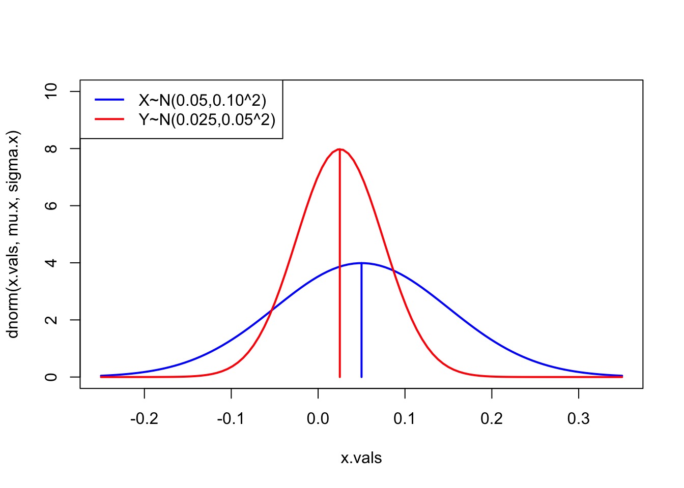
- Comment on the risk-return tradeoffs for the two stocks.
The return distribution for Microsoft (asset X in blue) has a higher mean and larger standard deviation (return uncertainty) than the return distribution for Starbucks (asset Y in red). This reflects the often observed result that higher expected return comes with higher risk (uncertainty).
- Let \(R\) denote the simple monthly return on Microsoft stock and let \(W_0\) denote initial wealth to be invested over the month. Assume that \(R \sim N(0.04, (0.09)^{2}) \text{ and that } W_0 = \$100,000\).
- Determine the \(1\%\) and \(5\%\) value-at-risk (VaR) over the month on the investment. That is, determine the loss in investment value that may occur over the next month with \(1\%\) probability and with \(5\%\) probability.
## [1] -10804## [1] -16937So with 5% probability, we could lose $10,804 or more over the next month out of our initial $100,000 investment; with 1% probability, we could lose $16,937 or more.
- Let \(r\) denote the continuously compounded monthly return on Microsoft stock and let \(W_0\) denote initial wealth to be invested over the month. Assume that \(r \sim \text{ iid } N(0.04, (0.09)^2)\) and that \(W_0 = \$100,000\).
- Determine the \(1\%\) and \(5\%\) value-at-risk (VaR) over the month on the investment. That is, determine the loss in investment value that may occur over the next month with \(1\%\) probability and with \(5\%\) probability. (Hint: compute the \(1\%\) and \(5\%\) quantile from the Normal distribution for \(r\) and then convert continuously compounded return quantile to a simple return quantile using the transformation)
## [1] -10241## [1] -15580When continuously compounded returns are normally distributed, with 5% probabilitywe could lose $10,241 or more over the next month out of our initial $100,000 investment; with 1% probability, we could lose $15,580 or more. Notice that these losses are smaller than when we assumed that simple returns are normally distributed. This is due to the fact that when continuously compounded returns are normally distributed, simple gross returns are log-normally distributed and the log-normal distribution has a positive skewness (hence shorter left tail). That is, the log-normal distribution has less probability in the left tail than the normal distribution.
- Determine the \(1\%\) and \(5\%\) value-at-risk (VaR) over the year on the investment. Hint: to answer this question, you must determine the normal distribution that applies to the annual (12 month) continuously compounded return. This was done as an example in class.
To compute the VaR on the annual investment, we must determine the distribution of the annual return. Assuming that that \(r \sim \text{iid } N(0.04, (0.09)^2)\), it follows that the annual continuously compounded return is also normally distributed with mean \(12\times(0.04) = 0.48\) and standard deviation \(\sqrt{12}\times (0.09) = 0.3118\) (see calculations at the end of the lecture notes on review of probability). The 5% and 1% VaR values are computed using
mu.r.12 = 12*mu.r
sigma.r.12 = sqrt(12)*sigma.r
VaR.05.12 = W0*(exp(qnorm(0.05, mu.r.12, sigma.r.12)) - 1)
VaR.05.12
## [1] -3228## [1] -21752With 5% probability we could lose $3,228 or more over the next year out of our initial $100,000 investment; with 1% probability, we could lose $21,752 or more.
- In this question, you will examine the chi-square and Student’s t distributions.
- On the same graph, plot the probability curves of chi-squared distributed random variables with 1, 2, 5 and 10 degrees of freedom. Use different colors and line styles for each curve.
A chi-square random variable with v degrees of freedom is defined as the sum of \(v\) squared independent standard normal random variables \(X = Z_{1}^{2} + Z_{2}^{2} + \cdots + Z_{v}^{2}\). The following shows a plot of the chi-square pdf for different values of \(v\).
x.vals = seq(0, 20, length=100)
plot(x.vals, dchisq(x.vals, df=1), type="l", lwd=2, lty=1, col=1, ylab="pdf", xlab="x")
lines(x.vals, dchisq(x.vals, df=2), lwd=2, lty=2, col=2)
lines(x.vals, dchisq(x.vals, df=5), lwd=2, lty=3, col=3)
lines(x.vals, dchisq(x.vals, df=10), lwd=2, lty=4, col=4)
legend(x="topright", legend=c("df=1", "df=2", "df=5", "df=10"), lwd=2, lty=1:4, col=1:4)
title("Chi-square distributions")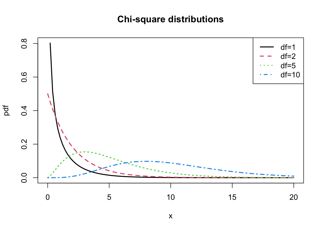
For small values of \(v\), the pdf is concentrated close to zero. For larger values of \(v\), the distribution becomes more spread out and actually starts to look normal.
- On the same graph, plot the probability curves of Student’s t distributed random variables with 1, 2, 5 and 10 degrees of freedom. Also include the probability curve for the standard normal distribution. Use different colors and line styles for each curve.
A Student’s t random variable is defined as a standard normal random variable divided by the square root of a chi-square random variable divided by its degrees of freedom:
\[ Y = \frac{Z}{\sqrt{X/4}}, Z \sim N(0,1), X \sim \chi_{v}^{2} \] where \(Z\) is independent of \(X\). following shows a plot of the Student’s t pdf for different values of \(v\).
x.vals = seq(-4, 4, length=100)
plot(x.vals, dt(x.vals, df=1), type="l", lwd=2, lty=1, col=1,
     ylab="pdf", xlab="x", ylim=c(0, 0.4))
lines(x.vals, dt(x.vals, df=2), lwd=2, lty=2, col=2)
lines(x.vals, dt(x.vals, df=5), lwd=2, lty=3, col=3)
lines(x.vals, dt(x.vals, df=10), lwd=2, lty=4, col=4)
legend(x="topright", legend=c("df=1", "df=2", "df=5", "df=10"), lwd=2, lty=1:4, col=1:4)
title("Student's t distributions")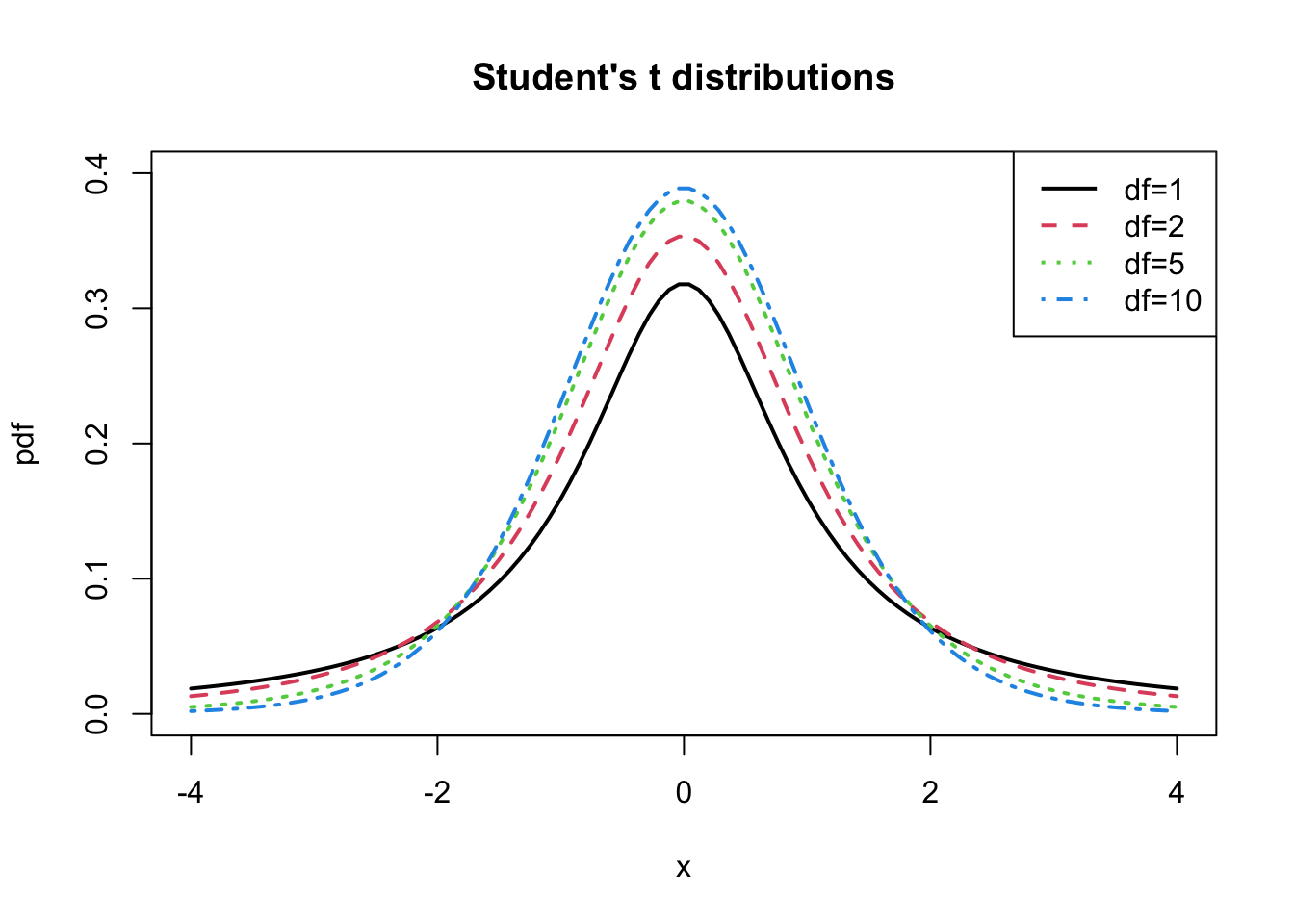
The distribution is centered at zero like the standard normal, but has fatter tails than the normal. As \(v\) gets bigger, the distribution gets closer to the standard normal distribution.
- Consider the following joint distribution of \(X\) and \(Y\):
| X-Y | 1 | 2 | 3 |
|---|---|---|---|
| 1 | 0.1 | 0.2 | 0 |
| 2 | 0.1 | 0 | 0.2 |
| 3 | 0 | 0.1 | 0.3 |
Find the marginal distributions of \(X\) and \(Y\). Using these distributions, compute \(E[X]\), \(var(X)\), \(SD(X)\), \(E[Y]\), \(var(Y)\) and \(SD(Y)\).
Compute \(\mathrm{COV}(X,Y)\) and \(\mathrm{CORR}(X,Y)\)
Are \(X\) and \(Y\) independent? Fully justify your answer.
This is tedious to do in R. See the calculations in the Excel spreadsheet 424lab2solutions.xls.
- Consider a one month investment in two Northwest stocks: Amazon and Costco. Suppose you buy Amazon and Costco at the end of September at \(P_{A,t-1} = \$38.23, P_{C,t-1} = \$41.11\) and then sell at the end of the October for \(P_{A,t} = \$41.29, P_{C,t} = \$41.74\) . (Note: these are actual closing prices for 2004 taken from Yahoo!)
First define the vector of prices
- What are the simple monthly returns for the two stocks?
## [1] 0.08004## [1] 0.01532- What are the continuously compounded returns for the two stocks?
## [1] 0.077## [1] 0.01521- Suppose Costco paid a \(\$0.10\) per share cash dividend at the end of October. What is the monthly simple total return on Costco? What is the monthly dividend yield?
## [1] 0.01776## [1] 0.002432- Suppose the monthly returns on Amazon and Costco from question (a) above are the same every month for 1 year. Compute the simple annual returns as well as the continuously compounded annual returns for the two stocks.
## [1] 1.519## [1] 0.924- At the end of September, 2004, suppose you have \(\$10,000\) to invest in Amazon and Costco over the next month. If you invest \(\$8,000\) in Amazon and \(\$2,000\) in Costco, what are your portfolio shares, \(x_A \text{ and } x_C\). (Assume partial share purchases are possible)
## [1] 0.8 0.2- Continuing with the previous question, compute the monthly simple return and the monthly continuously compounded return on the portfolio. Assume that Costco does not pay a dividend.
## [1] 0.06710 0.06494- Consider an investment in a foreign stock (e.g. a stock trading on the London stock exchange) by a U.S. national (domestic investor). The domestic investor takes U.S. dollars, converts them to the foreign currency (e.g. British Pound) via the exchange rate (price of foreign currency in U.S. dollars) and then purchases the foreign stock using the foreign currency. When the stock is sold, the proceeds in the foreign currency must then be converted back to the domestic currency. To be more precise, consider the information in the table below:
| Time | Cost of 1 Pound | Value of UK Shares | Value in U.S. $ |
|---|---|---|---|
| 0 | $1.50 | £40 | 1.5*40 = 60 |
| 1 | $1.30 | £45 | 1.3*45 = 58.5 |
- Compute the simple rate of return, Re, from the prices of foreign currency.
## [1] -0.1333- Compute the simple rate of return, Ruk, from the UK stock prices.
## [1] 0.125- Compute the simple rate of return, Rus, from the prices in US dollars.
## [1] -0.025- What is the relationship between Rus, Ruk and Re?
The US return can be expressed as
\[ R_{US}=\frac{P_{1,US} - P_{0,US}}{P_{0,US}} = \frac{E_1 \times P_{1,UK} - E_0 \times P_{0,UK}}{E_0 \times P_{0,UK}} = \frac{E_1 \times P_{1,UK}}{E_0 \times P_{0,UK}} \] where \(E\) denotes the exchange rate (price of foreign currency in US dollars). Next, note that
\[ \frac{E_1}{E_0} = 1 + R_E, \frac{P_{1,UK}}{P_{0,UK}} = 1 + R_{UK} \] where
\[ R_E = \frac{E_1-E_0}{E_0}, R_{UK} = \frac{P_{1,UK} - P_{0,UK}}{P_{0,UK}} \] Then we have the relationship
\[ R_{US} = (1 + R_E) \times (1 + R_{UK}) - 1 \] Here is the check in R:
## [1] -0.025- Let \(R_t\) denote the simple monthly return and assume that \(R_t \sim N(\mu, \sigma^2)\). Consider the 2-period simple return \(R_t(2) = (1 + R_t)(1 + R_{t-1}) - 1\).
- Assuming that \(\mathrm{COV}(R_t, R_{t-1}) = 0\), show that \(E[R_t R_{t-1}] = \mu^2\) . Hint: Use \(\mathrm{COV}(R_t, R_{t-1}) = E[R_t R_{t-1}] - E[R_t]E[R_{t-1}]\) .
Because \(R_t \sim \mathrm{iid} ~ N(\mu, \sigma^2)\)
\[ 0 = \mathrm{cov}(R_t,R_{t-1}) = E[R_t R_{t-1}] - E[R_t]E[R_{t-1}] \Rightarrow E[R_t R_{t-1}] = E[R_t]E[R_{t-1}] = \mu^2 \]
- Show that \(E[R_t(2)] = (1 + \mu)^2 - 1\)
\[\begin{align*} E[R_t(2)] & = E[(1 + R_t)(1 + R_{t-1}) - 1] = E[1 + R_{t-1} + R_t + R_tR_{t-1}] = 1 + E[R_{t-1}] + E[R_t] + E[R_tR_{t-1}] - 1\\ & = 1+ \mu + \mu +\mu^2 - 1= 1 + 2\mu + \mu^2 - 1\\ & = (1 + \mu)^2 - 1 \end{align*}\]
- Is \(R_t(2)\) normally distributed? Why or why not?
\(R_t(2)\) is not normally distributed because \(R_t \times R_{t-1}\) is not normally distributed.
References
Amemiya, T. 1994. Introduction to Statistics and Econometrics. Cambridge, MA.: Harvard University Press.
Carmona, R. 2014. Statistical Analysis of Financial Data in R, Second Edition. New York: Springer.
Dalgaard, P. 2002. Introductory Statistics with R. Springer.
DeGroot, M. H., and M. J. Schervish. 2011. Probability and Statistics, 4th Edition. Pearson.
Goldberger, A. S. 1991. A Course in Econometrics. Cambridge, MA.: Harvard University Press.
Pfaff, B. 2013. Financial Risk Modelling and Portfolio Optimization with R. Chichester, UK.: Wiley.
Ruppert, D., and D. S. Matteson. 2015. Statistics and Data Analysis for Financial Engineering with R Examples. New York: Springer.
Verzani, J. 2005. Using R for Introductory Statistics. Boca Raton: Chapman & Hall/CRC.
If \(P_{t+1}\) is a positive random variable such that \(\ln P_{t+1}\) is normally distributed then \(P_{t+1}\) has a log-normal distribution.↩︎
An inflection point is a point where a curve goes from concave up to concave down, or vice versa.↩︎
The inverse function of \(F_{X}\) , denoted \(F_{X}^{-1},\) has the property that \(F_{X}^{-1}(F_{X}(x))=x.\) \(F_{X}^{-1}\) will exist if \(F_{X}\) is strictly increasing and is continuous.↩︎
Using R, \(z_{.05}=\mathrm{qnorm}(0.05)=-1.645\).↩︎