10 Modeling Daily Returns with the GARCH Model

Updated: May 12, 2021

Copyright © Eric Zivot 2016

Outline

1. Motivation
   1. Review stylized facts of daily return data and contrast with monthly returns
   2. Modeling daily returns is most useful for short term risk analysis of assets and portfolios using volatility and VaR
   3. CER model captures most stylized facts of monthly returns but not daily returns
   4. Need a model for time varying volatility
   5. Engle’s ARCH model captures stylized facts of daily returns and he was awarded Nobel prize in economics partially for this model.
2. Engle’s ARCH Model
   1. Start with ARCH(1) process
   2. State assumptions and derive properties
   3. Show simulated values and do reality check against actual data
   4. Introduce rugarch R package
   5. General ARCH(p) process
3. Bollerslev’s GARCH(1,1) process
   1. No need to go beyond GARCH(1,1)
   2. Give assumptions and derive basic properties
   3. Show simulated values and do reality check against actual data
   4. GARCH(1,1) with Student t errors
   5. Show simulated values and do reality check against actual data
4. Maximum Likelihood Estimation
   1. Overview of the technique of MLE
   2. Illustration with CER model and GARCH(1,1)
   3. Numerical optimization
   4. Asymptotic properties
   5. Calculating standard errors
5. Maximum likelihood estimation of ARCH and GARCH models
   1. GARCH(1,1) log-likelihood function
6. Forecasting Conditional Volatility from GARCH(1,1)
   1. Forecasting algorithm
   5. Multiperiod
7. Conditional VaR
   1. unconditional vs. conditional VaR
   2. 1-day ahead VaR forecast
   3. h-day ahead VaR forecast

In chapter 5, it was shown that daily asset returns have some features in common with monthly asset returns and some not. In particular, daily returns have empirical distributions with much fatter tails than the normal distribution and daily returns are not independent over time. Absolute and squared returns are positively autocorrelated and the correlation dies out very slowly. Daily volatility appears to be autocorrelated and, hence, predictable. In this chapter we present a model of daily asset returns, Robert Engle’s (ARCH) model, that can capture these stylized facts that are specific to daily returns. The ARCH model is one of the most important models in the field of financial econometrics, and its creator Robert Engle won the Nobel Prize in Economics in part for his work on the ARCH model and its variants.

The R packages used in this chapter are IntroCompFinR, rugarch and xts. Make sure these package are installed and loaded before running the R examples in this chapter.

• Why do we care about time varying volatility? Volatility is a standard measure of asset risk and if volatility varies over time then asset risk also varies over time. In periods of low volatility, asset risk is low and in periods of high volatility asset risk is high. Time varying volatility also impacts the risk measure value-at-risk (VaR), which gives the dollar loss that could occur over a period of time with a given probability. Volatility is an important driver for the price of call and put options as well as other derivative securities. That volatility is predictable has important implications for accurate pricing models for options and derivatives.
• Why do we care about the predictability of volatility? We can forecast future values of volatility. This allows us to forecast VaR on an asset or portfolio.

10.1 Engle’s ARCH Model

• Goal: create a simple time series model that captures the basic stylized facts of daily return data
• Foundation of the field of financial econometrics

10.1.1 The ARCH(1) Model

Let $R_{t}$ denote the continuously compounded daily return on an asset. The CER model for $R_{t}$ can be expressed in the form: $$\begin{eqnarray} R_{t} & = & \mu+\epsilon_{t},\,t=1,\ldots,T,\tag{10.1}\\ \epsilon_{t} & = & \sigma z_{t},\tag{10.2}\\ z_{t} & \sim & iid\,N(0,1).\tag{10.3} \end{eqnarray}$$ Here, the unexpected return $\epsilon_{t}$ is expressed as $\sigma z_{t}$ where $\sigma$ is the unconditional volatility of $\epsilon_{t}$, which is assumed to be constant, and $z_{t}=\epsilon_{t}/\sigma$ is the standardized unexpected return. In (10.1)-(10.3), $R_{t}\sim iid\,N(\mu,\sigma^{2})$ which is not a good model for daily returns given the stylized facts. The ARCH(1) model for $R_{t}$ has a similar form: $$\begin{eqnarray} R_{t} & = & \mu+\epsilon_{t},\,t=1,\ldots,T,\tag{10.4}\\ \epsilon_{t} & = & \sigma_{t}z_{t},\tag{10.5}\\ \sigma_{t}^{2} & = & \omega+\alpha_{1}\epsilon_{t-1}^{2},\tag{10.6}\\ z_{t} & \sim & iid\,N(0,1),\tag{10.7}\\ \omega>0, & & 0\leq\alpha_{1}<1.\tag{10.8} \end{eqnarray}$$

In the ARCH(1), the unexpected return $\epsilon_{t}$ is expressed as $\sigma_{t}z_{t}$ where $\sigma_{t}$ is the conditional (time $t$ dependent) volatility of $\epsilon_{t}$. Hence, the ARCH(1) model extends the CER model to allow for time varying conditional volatility $\sigma_{t}.$

In the ARCH(1) model (10.4) - (10.8), the restrictions $\omega>0$ and $0\leq\alpha_{1}<1$ are required to ensure that $\sigma_{t}^{2}>0$ and that $\{R_{t}\}$ is a covariance stationary time series. Equation (10.6) shows that the return variance at time $t$, $\sigma_{t}^{2}$ is a positive linear function of the squared unexpected return at time $t-1$, $\epsilon_{t-1}^{2}$. This allows the magnitude of yesterday’s return to influence today’s return variance and volatility. In particular, a large (small) value of $\epsilon_{t-1}^{2}$ leads to a large (small) value of $\sigma_{t}^{2}$. This feedback from $\epsilon_{t-1}^{2}$ to $\sigma_{t}^{2}$ can explain some of the volatility clustering observed in daily returns.

10.1.1.1 Statistical properties of the ARCH(1) Model

Let $I_{t}=\{R_{t},R_{t-1},\ldots,R_{1}\}$ denote the information set at time $t$ (conditioning set of random variables) as described in Chapter 4. As we shall show below, the ARCH(1) model (10.4) - (10.8) has the following statistical properties:

1. $E(\epsilon_{t}|I_{t})=0,$ $E(\epsilon_{t})=0$.
2. $\mathrm{var}(R_{t}|I_{t})=E(\epsilon_{t}^{2}|I_{t})=\sigma_{t}^{2}$.
3. $\mathrm{var}(R_{t})=E(\epsilon_{t}^{2})=E(\sigma_{t}^{2})=\omega/(1-\alpha_{1})$.
4. $\{R_{t}\}$ is an uncorrelated process: $\mathrm{cov}(R_{t},R_{t-k})=E(\epsilon_{t}\epsilon_{t-j})=0$ for $k>0$.
5. The distribution of $R_{t}$ conditional on $I_{t-1}$ is normal with mean $\mu$ and variance $\sigma_{t}^{2}$.
6. The unconditional (marginal) distribution of $R_{t}$ is not normal and $\mathrm{kurt}(R_{t})\geq3$.
7. $\{R_{t}^{2}\}$ and $\{\epsilon_{t}^{2}\}$ have a covariance stationary AR(1) model representation. The persistence of the autocorrelations is measured by $\alpha_{1}.$

These properties of the ARCH(1) model match many of the stylized facts of daily asset returns.

It is instructive to derive each of the above properties as the derivations make use of certain results and tricks for manipulating conditional expectations. First, consider the derivation for property 1. Because $\sigma_{t}^{2}=\omega+\alpha_{1}\epsilon_{t-1}^{2}$ depends on information dated $t-1$, $\sigma_{t}^{2}\in I_{t-1}$ and so $\sigma_{t}^{2}$ may be treated as a constant when conditioning on $I_{t-1}.$ Hence, $$E(\epsilon_{t}|I_{t})=E(\sigma_{t}z_{t}|I_{t-1})=\sigma_{t}E(z_{t}|I_{t-1})=0.$$ The last equality follows from that fact that $z_{t}\sim iid\,N(0,1)$ which implies that $z_{t}$ is independent of $I_{t-1}$ and so $E(z_{t}|I_{t-1})=E(z_{t})=0$. By iterated expectations, it follows that $$E(\epsilon_{t})=E(E(\epsilon|I_{t-1}))=E(0)=0.$$ The derivation of the second property uses similar computations: $$\mathrm{var}(R_{t}|I_{t})=E((R_{t}-\mu)^{2}|I_{t-1})=E(\epsilon_{t}^{2}|I_{t})=E(\sigma_{t}^{2}z_{t}^{2}|I_{t-1})=\sigma_{t}^{2}E(z_{t}^{2}|I_{t-1})=\sigma_{t}^{2},$$ where the last equality uses the result $E(z_{t}^{2}|I_{t-1})=E(z_{t}^{2})=1$.

To derive property 3, first note that by iterated expectations and property 2 $$\mathrm{var}(R_{t})=E(\epsilon_{t}^{2})=E(E(\epsilon_{t}^{2}|I_{t}))=E(\sigma_{t}^{2}).$$

Next, using (10.6) we have that $$E(\sigma_{t}^{2})=\omega+\alpha_{1}E(\epsilon_{t-1}^{2}).$$ Now use the fact that $\{R_{t}\}$, and hence $\{\epsilon_{t}\}$, is covariance stationary which implies that $E(\epsilon_{t}^{2})=E(\epsilon_{t-1}^{2})=E(\sigma_{t}^{2})$ so that $$E(\sigma_{t}^{2})=\omega+\alpha_{1}E(\sigma_{t}^{2}).$$ Solving for $E(\sigma_{t}^{2})$ then gives $$\mathrm{var}(R_{t})=E(\sigma_{t}^{2})=\frac{\omega}{1-\alpha_{1}}.$$

For the fourth property, first note that $$\mathrm{cov}(R_{t},R_{t-k})=E((R_{t}-\mu)(r_{t-j}-\mu))=E(\epsilon_{t}\epsilon_{t-k})=E(\sigma_{t}z_{t}\sigma_{t-j}z_{t-j}).$$ Next, by iterated expectations and the fact that $z_{t}\sim iid\,N(0,1)$ we have $$E(\sigma_{t}z_{t}\sigma_{t-j}z_{t-j})=E(E(\sigma_{t}z_{t}\sigma_{t-j}z_{t-j}|I_{t-1}))=E(\sigma_{t}\sigma_{t-j}z_{t-j}E(z_{t}|I_{t-1}))=0,$$ and so $\mathrm{cov}(R_{t},R_{t-k})=0$.

To derive the fifth property, write $R_{t}=\mu+\epsilon_{t}=\mu+\sigma_{t}z_{t}.$ Then, conditional on $I_{t-1}$ and the fact that $z_{t}\sim iid\,N(0,1)$ we have $$R_{t}|I_{t-1}\sim N(\mu,\sigma_{t}^{2}).$$

The sixth property has two parts. To see that the unconditional distribution of $R_{t}$ is not a normal distribution, it is useful to express $R_{t}$ in terms of current and past values of $z_{t}$ . Start with $$R_{t}=\mu+\sigma_{t}z_{t}.$$ From (10.6), $\sigma_{t}^{2}=\omega+\alpha_{1}\epsilon_{t-1}^{2}=\omega+\alpha_{1}\sigma_{t-1}^{2}z_{t-1}^{2}$ which implies that $\sigma_{t}=(\omega+\alpha_{1}\sigma_{t-1}^{2}z_{t-1}^{2})^{1/2}$. Then $$R_{t}=\mu+(\omega+\alpha_{1}\sigma_{t-1}^{2}z_{t-1}^{2})^{1/2}z_{t}.$$

Even though $z_{t}\sim iid\,N(0,1)$, $R_{t}$ is a complicated nonlinear function of $z_{t}$ and past values of $z_{t}^{2}$ and so $R_{t}$ cannot be a normally distributed random variable. Next, to see that $\mathrm{kurt}(R_{t})\geq3$ first note that $$\begin{equation} \mathrm{kurt}(R_{t})=\frac{E((R_{t}-\mu)^{4})}{\mathrm{var}(R_{t})^{2}}=\frac{E(\epsilon_{t}^{4})}{\omega^{2}/(1-\alpha_{1})^{2}}\tag{10.9} \end{equation}$$ Now by iterated expectations and the fact that $E(z_{t}^{4})=3$ $$E(\epsilon_{t}^{4})=E(E(\sigma_{t}^{4}z_{t}^{4}|I_{t-1}))=E(\sigma_{t}^{4}E(z_{t}^{4}|I_{t-1}))=3E(\sigma_{t}^{4}).$$ Next, using $$\begin{eqnarray*} \sigma_{t}^{4} & = & (\sigma_{t}^{2})^{2}=(\omega+\alpha_{1}\epsilon_{t-1}^{2})^{2}\\ & = & \omega^{2}+2\omega\alpha_{1}\epsilon_{t-1}^{2}+\alpha_{1}^{2}\epsilon_{t-1}^{4} \end{eqnarray*}$$ we have $$\begin{eqnarray*} E(\epsilon_{t}^{4}) & = & 3E(\omega^{2}+2\omega\alpha_{1}\epsilon_{t-1}^{2}+\alpha_{1}^{2}\epsilon_{t-1}^{4})\\ & = & 3\omega^{2}+6\omega\alpha_{1}E(\epsilon_{t-1}^{2})+3\alpha_{1}^{2}E(\epsilon_{t-1}^{4}). \end{eqnarray*}$$ Since $\{R_{t}\}$ is covariance stationary it follows that $E(\epsilon_{t-1}^{2})=E(\epsilon_{t}^{2})=E(\sigma_{t}^{2})=\omega/(1-\alpha_{1})$ and $E(\epsilon_{t-1}^{4})=E(\epsilon_{t}^{4})$. Hence $$\begin{eqnarray*} E(\epsilon_{t}^{4}) & = & 3\omega^{2}+6\omega\alpha_{1}(\omega/(1-\alpha_{1}))+3\alpha_{1}^{2}E(\epsilon_{t}^{4})\\ & = & 3\omega^{2}\left(1+2\frac{\alpha_{1}}{1-\alpha_{1}}\right)+3\alpha_{1}^{2}E(\epsilon_{t}^{4}). \end{eqnarray*}$$ Solving for $E(\epsilon_{t}^{4})$ gives $$E(\epsilon_{t}^{4})=\frac{3\omega^{2}(1+\alpha_{1})}{(1-\alpha_{1})(1-3\alpha_{1}^{2})}.$$ Because $0\leq\alpha_{1}<1$, in order for $E(\epsilon_{t}^{4})<\infty$ it must be the case that $1-3\alpha_{1}^{2}>0$ which implies that $0\leq\alpha_{1}^{2}<\frac{1}{3}$ or $0\leq\alpha_{1}<0.577$. Substituting the above expression for $E(\epsilon_{t}^{4})$ into (10.9) then gives $$\begin{eqnarray*} \mathrm{kurt}(R_{t}) & = & \frac{3\omega^{2}(1+\alpha_{1})}{(1-\alpha_{1})(1-3\alpha_{1}^{2})}\times\frac{(1-\alpha_{1})^{2}}{\omega^{2}}\\ & = & 3\frac{1-\alpha_{1}^{2}}{1-3\alpha_{1}^{2}}\geq3. \end{eqnarray*}$$ Hence, if returns follow an ARCH(1) process with $\alpha_{1}>0$ then $\mathrm{kurt}(R_{t})>3$ which implies that the unconditional distribution of returns has fatter tails than the normal distribution.

To show the last property, add $\epsilon_{t-1}^{2}$ to both sides of (10.6) to give $$\begin{eqnarray*} \epsilon_{t}^{2}+\sigma_{t}^{2} & = & \omega+\alpha_{1}\epsilon_{t-1}^{2}+\epsilon_{t}^{2}\Rightarrow\\ \epsilon_{t}^{2} & = & \omega+\alpha_{1}\epsilon_{t-1}^{2}+\epsilon_{t}^{2}-\sigma_{t}^{2}\\ & = & \omega+\alpha_{1}\epsilon_{t-1}^{2}+v_{t}, \end{eqnarray*}$$ where $v_{t}=\epsilon_{t}^{2}-\sigma_{t}^{2}$ is a mean-zero and uncorrelated error term. Hence, $\epsilon_{t}^{2}$ and $R_{t}^{2}$ follow an AR(1) process with positive autoregressive coefficient $\alpha_{1}.$ The autocorrelations of $R_{t}^{2}$ are $$\mathrm{cor}(R_{t}^{2},R_{t-j}^{2})=\alpha_{1}^{j}\,for\,j>1,$$ which are positive and decay toward zero exponentially fast as $j$ gets large. Here, the persistence of the autocorrelations is measured by $\alpha_{1}.$

Example 10.1 (Simulate an ARCH(1) model using brute force)

To be completed

$\blacksquare$

10.1.1.2 The rugarch package

• Give a brief introduction to the rugarch package

Example 10.2 ( Simulate an ARCH(1) model using rugarch )

Consider the simple ARCH(1) model for returns $$\begin{align*} R_{t} & =\varepsilon_{t}=\sigma_{t}z_{t},\text{ }z_{t}\sim iid\text{ }N(0,1)\\ \sigma_{t}^{2} & =0.5+0.5R_{t-1}^{2} \end{align*}$$ Here, $\alpha_{1}=0.5<1$ so that $R_{t}$ is covariance stationary and $\bar{\sigma}^{2}=\omega/(1-\alpha_{1})=0.5/(1-0.5)=1.$ Using (10.9), $$\mathrm{kurt}(R_{t})=3\frac{1-\alpha_{1}^{2}}{1-3\alpha_{1}^{2}}=3\frac{1-(0.5)^{2}}{1-3(0.5)^{2}}=9,$$ so that the distribution of $R_{t}$ has much fatter tails than the normal distribution.

The rugarch functions ugarchspec() and ugarchpath() can be used to simulate $T=1000$ values of $R_{t}$ and $\sigma_{t}$ from this model.⁵³ The ARCH(1) model is specified using the ugarchpath() function as follows

library(rugarch)
library(PerformanceAnalytics)
arch1.spec = ugarchspec(variance.model = list(garchOrder=c(1,0)),
                        mean.model = list(armaOrder=c(0,0)),
                        fixed.pars=list(mu = 0, omega=0.5, alpha1=0.5))

The argument fixed.pars is a list whose components give the ARCH(1) model parameters. The names of the list components match the parameters from the ARCH(1) model: mu is $\mu$, omega is $\omega$, and alpha1 is $\alpha_{1}.$ Simulated values of $R_{t}$ and $\sigma_{t}$ are produced using the ugarchpath() function taking as input the "uGARCHspec" object arch1.spec and the number of simulations, n.sim=1000, to produce:

set.seed(123)
arch1.sim = ugarchpath(arch1.spec, n.sim=1000)
class(arch1.sim)

## [1] "uGARCHpath"
## attr(,"package")
## [1] "rugarch"

slotNames(arch1.sim)

## [1] "path"  "model" "seed"

names(arch1.sim@path)

## [1] "sigmaSim"  "seriesSim" "residSim"

The object arch1.sim is an Sv4 object of class uGARCHpath for which there are sigma, fitted, quantile, show and plot methods.⁵⁴ The path slot is a list which contains the simulated values of $\sigma_{t},$ $R_{t}$ and $\varepsilon_{t}=R_{t}-\mu_{t}$ as matrix objects. The method functions sigma() and fitted() extract $\sigma_{t}$ and $\mu_{t},$ respectively. Invoking the plot() method produces a menu of plot choices

Individual plots can be produced directly by specifying the plot number in the call to plot(). For example, Figure 10.1 shows the plots of the simulated values for $R_{t}$ and $\sigma_{t}$ created with

library(sp)
graphics::par(mfrow=c(2,1))
   sp::plot(arch1.sim, which=2)
   sp::plot(arch1.sim, which=1)

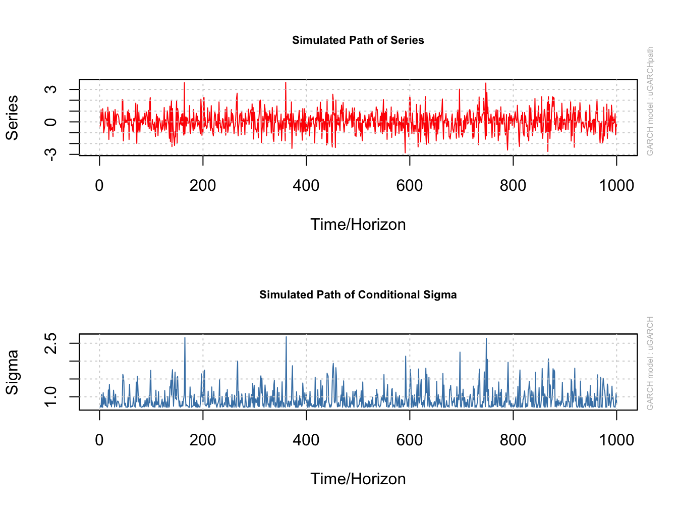
Figure 10.1: Simulated values from ARCH(1) process. Top panel: simulated values of $R_{t}$. Bottom panel: simulated values of $\sigma_{t}.$

graphics::par(mfrow=c(1,1))

Figure 10.2 shows the sample autocorrelations of $R_{t}$ and $R_{t}^{2}$. As expected returns are uncorrelated whereas $R_{t}^{2}$ has autocorrelations described by an AR(1) process with positive autoregressive coefficient$.$

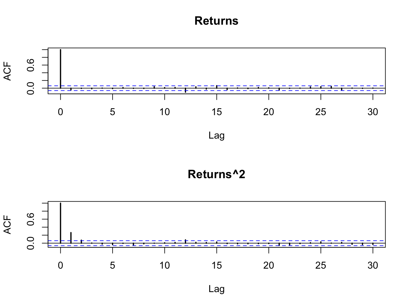
Figure 10.2: SACFs for $R_{t}$(top panel) and $R_{t}^{2}$ (bottom panel) from simulated ARCH(1) model.

The sample variance and excess kurtosis of the simulated returns are

as.numeric(var(arch1.sim@path$seriesSim))

## [1] 0.876

kurtosis(arch1.sim@path$seriesSim)

## [1] 0.65

The sample variance is very close to the unconditional variance $\bar{\sigma}^{2}=0.2$, and the sample excess kurtosis is very close to the ARCH(1) excess kurtosis of $6$.

$\blacksquare$

10.1.2 The ARCH(p) Model

The ARCH(p) model extends the autocorrelation structure of $R_{t}^{2}$ and $\epsilon_{t}^{2}$ in the ARCH(1) model (10.4) - (10.6) to that of an AR(p) process by adding $p$ lags of $\epsilon_{t}^{2}$ to the dynamic equation for $\sigma_{t}^{2}:$ $$\begin{eqnarray} \sigma_{t}^{2} & = & \omega+\alpha_{1}\epsilon_{t-1}^{2}+\alpha_{2}\epsilon_{t-2}^{2}+\cdots+\alpha_{p}\epsilon_{t-p}^{2},\tag{10.10} \end{eqnarray}$$ In order for $\sigma_{t}^{2}$ to be positive we need to impose the restrictions $$\begin{equation} \omega>0,\,\alpha_{1}\geq0,\,\alpha_{2}\geq0,\,\ldots,\alpha_{p}\geq0.\tag{10.11} \end{equation}$$ In addition, for $\{R_{t}\}$ to be a covariance stationary time series we must have the restriction $$\begin{equation} 0\leq\alpha_{1}+\alpha_{2}+\cdots+\alpha_{p}<1.\tag{10.12} \end{equation}$$ The statistical properties of the ARCH(p) model are the same as those for the ARCH(1) model with the following exceptions. The unconditional variance of $\{R_{t}\}$ is $$\begin{equation} \mathrm{var}(R_{t})=E(\epsilon_{t}^{2})=E(\sigma_{t}^{2})=\omega/(1-\alpha_{1}-\alpha_{2}-\cdots-\alpha_{p}),\tag{10.13} \end{equation}$$ and $\{R_{t}^{2}\}$ and $\{\epsilon_{t}^{2}\}$ have a covariance stationary AR(p) model representation whose autocorrelation persistence is measured by the sum of the ARCH coefficients $\alpha_{1}+\alpha_{2}+\cdots+\alpha_{p}$.

The ARCH(p) model is capable of creating a much richer autocorrelation structure for $R_{t}^{2}$. In the ARCH(1) model, the autocorrelations of $R_{t}^{2}$ decay to zero fairly quickly whereas the sample autocorrelations shown in Figure 10.2 decay to zero very slowly. In the ARCH(p) model, because of the restrictions (10.11) and (10.12), for large values of $p$ the dynamics of $\sigma_{t}^{2}$ from (10.10) can more closely mimic the observed autocorrelations of actual daily returns.

Example 10.3 ( Simulate ARCH(p) model using rugarch )

To be completed. Simulate long order AR(10) to show difference with ARCH(1). Make sum of ARCH coefficients equal to 0.9

$\blacksquare$

10.2 Bollerslev’s GARCH Model

An important extension of the ARCH(p) model proposed by Bollerslev (1986) replaces the AR$(p)$ representation of $\sigma_{t}^{2}$ in (10.10) with an ARMA($p,q$) formulation giving the GARCH(p,q) model: $$\begin{align} \sigma_{t}^{2} & =\omega+\sum_{i=1}^{p}\alpha_{i}\varepsilon_{t-i}^{2}+\sum_{j=1}^{q}\beta_{j}\sigma_{t-j}^{2}\tag{10.14} \end{align}$$ In order for $\sigma_{t}^{2}>0,$ it is assumed that $\omega>0$ and the coefficients $\alpha_{i}$ $(i=0,\cdots,p)$ and $\beta_{j}$ $(j=1,\cdots,q)$ are all non-negative.⁵⁵ When $q=0$, the GARCH(p,q) model (10.14) reduces to the ARCH(p) model. In general, the GARCH($p,q)$ model can be shown to be equivalent to a particular ARCH($\infty)$ model.

Usually the GARCH(1,1) model, $$\begin{equation} \sigma_{t}^{2}=\omega+\alpha_{1}\varepsilon_{t-1}^{2}+\beta_{1}\sigma_{t-1}^{2},\tag{10.15} \end{equation}$$ with only three parameters in the conditional variance equation is adequate to obtain a good model fit for daily asset returns. Indeed, Hansen and Lund (2004) provided compelling evidence that is difficult to find a volatility model that outperforms the simple GARCH(1,1). Hence, for many purposes the GARCH(1,1) model is the de facto volatility model of choice for daily returns.

10.2.1 Statistical Properties of the GARCH(1,1) Model

The statistical properties of the GARCH(1,1) model are derived in the same way as the properties of the ARCH(1) model and are summarized below:

1. $\{R_{t}\}$ is a covariance stationary and ergodic process provided $\alpha_{1}+\beta_{1}<1$.
2. $\mathrm{v\mathrm{ar}}(R_{t})=E(\epsilon_{t}^{2})=E(\sigma_{t}^{2})=\omega/(1-\alpha_{1}-\beta_{1})=\bar{\sigma}^{2}.$
3. The distribution of $R_{t}$ conditional on $I_{t-1}$ is normal with mean $\mu$ and variance $\sigma_{t}^{2}$.
4. The unconditional (marginal) distribution of $R_{t}$ is not normal and $$\mathrm{kurt}(R_{t})=\frac{3(1+\alpha_{1}+\beta_{1})(1-\alpha_{1}-\beta_{1})}{1-2\alpha_{1}\beta_{1}-3\alpha_{1}^{2}-\beta_{1}^{2}}\geq3.$$
5. $\{R_{t}^{2}\}$ and $\{\varepsilon_{t}^{2}\}$ have an ARMA(1,1) representation $$\varepsilon_{t}^{2}=\omega+(\alpha_{1}+\beta_{1})\varepsilon_{t-1}^{2}+u_{t}-\beta_{1}u_{t-1},$$ with $u_{t}=\varepsilon_{t}^{2}-\sigma_{t}^{2}$. The persistence of the autocorrelations is given by $\alpha_{1}+\beta_{1}.$
6. $\sigma_{t}^{2}$ has an AR($\infty)$ representation $$\sigma_{t}^{2}=\frac{\omega}{1-\beta_{1}}+\alpha_{1}\sum_{j=0}^{\infty}\beta_{1}^{j}\varepsilon_{t-j-1}^{2}.$$

The derivations of these properties are left as end-of-chapter exercise.

• Need some comments here: more flexible autocorrelations structure for $R_{t}^{2}$ than ARCH(p) and with fewer parameters.

Example 10.4 (Simulate GARCH(1,1) model using rugarch)

Consider simulating $T=1000$ observations from the GARCH(1,1) model $$\begin{align*} R_{t} & =\varepsilon_{t}=\sigma_{t}z_{t},\text{ }z_{t}\sim iid\text{ }N(0,1)\\ \sigma_{t}^{2} & =0.01+0.07R_{t-1}^{2}+0.92\sigma_{t-1}^{2} \end{align*}$$ This process is covariance stationary since $\alpha_{1}+\beta_{1}=0.07+0.92=0.9<1,$ and $\bar{\sigma}^{2}=\omega/(1-\alpha_{1}-\beta_{1})=0.01/0.01=1.$ This GARCH(1,1) model has the same unconditional variance as the ARCH(5) model from the previous example but has much higher persistence. This model can be specified using the rugarch ugarchspec() function as follows:

garch11.spec = ugarchspec(variance.model = list(garchOrder=c(1,1)), 
                          mean.model = list(armaOrder=c(0,0)),
                          fixed.pars=list(mu = 0, omega=0.1, 
                                          alpha1=0.1, beta1 = 0.8))

This model has the same unconditional variance and persistence as the ARCH(5) model in the previous example. Simulated values for $R_{t}$ and $\sigma_{t},$ using the same random number seed as the ARCH(5) simulations, are created using

set.seed(123)
garch11.sim = ugarchpath(garch11.spec, n.sim=1000)

and are displayed in Figure xxx. The simulated GARCH(1,1) values of $R_{t}$ and $\sigma_{t}$ are quite different from the simulated ARCH(1) values. In particular, the simulated returns $R_{t}$ show fewer extreme values than the ARCH(1) returns and the simulated volatilities $\sigma_{t}$ values appear to show more persistence than the ARCH(1) volatilities. The sample autocorrelations in Figure xxx show the interesting result that $R_{t}^{2}$ exhibits little autocorrelation whereas $\sigma_{t}^{2}$ exhibits substantial positive autocorrelation.

sd(garch11.sim@path$seriesSim)

## [1] 0.963

kurtosis(garch11.sim@path$seriesSim)

## [1] 0.0443

$\blacksquare$

10.3 Maximum Likelihood Estimation

The estimation of the ARCH-GARCH model parameters is more complicated than the estimation of the CER model parameters. There are no simple plug-in principle estimators for the conditional variance parameters. Instead, an alternative estimation method called maximum likelihood (ML) is typically used to estimate the ARCH-GARCH parameters. This section reviews the ML estimation method and shows how it can be applied to estimate the ARCH-GARCH model parameters.

10.3.1 The Likelihood Function

Let $X_{1},\ldots,X_{T}$ be an iid sample with probability density function (pdf) $f(x_{t};\theta),$ where $\theta$ is a $(k\times1)$ vector of parameters that characterize $f(x_{t};\theta).$ For example, if $X_{t}\sim N(\mu,\sigma^{2})$ then $f(x_{t};\theta)=(2\pi\sigma^{2})^{-1/2}\exp\left(-\frac{1}{2\sigma^{2}}(x_{t}-\mu)^{2}\right)$ and $\theta=(\mu,\sigma^{2})^{\prime}.$  The joint density of the sample is, by independence, equal to the product of the marginal densities $$\begin{equation} f(x_{1},\ldots,x_{T};\theta)=f(x_{1};\theta)\cdots f(x_{T};\theta)=\prod_{t=1}^{T}f(x_{t};\theta).\tag{10.16} \end{equation}$$ The joint density is a $T$ dimensional function of the data $x_{1},\ldots,x_{T}$ given the parameter vector $\theta.$ The joint density satisfies⁵⁶ $$\begin{align*} f(x_{1},\ldots,x_{T};\theta) & \geq0,\\ \int\cdots\int f(x_{1},\ldots,x_{T};\theta)dx_{1}\cdots dx_{T} & =1. \end{align*}$$

The likelihood function is defined as the joint density treated as a function of the parameters $\theta:$ $$\begin{equation} L(\theta|x_{1},\ldots,x_{T})=f(x_{1},\ldots,x_{T};\theta)=\prod_{t=1}^{T}f(x_{t};\theta).\tag{10.17} \end{equation}$$ Notice that the likelihood function is a $k$ dimensional function of $\theta$ given the data $x_{1},\ldots,x_{T}.$ It is important to keep in mind that the likelihood function, being a function of $\theta$ and not the data, is not a proper pdf. It is always positive but $$\int\cdots\int L(\theta|x_{1},\ldots,x_{T})d\theta_{1}\cdots d\theta_{k}\neq1.$$

To simplify notation, let the vector $\mathbf{x}=(x_{1},\ldots,x_{T})^{\prime}$ denote the observed sample. Then the joint pdf and likelihood function may be expressed as $f(\mathbf{x};\theta)$ and $L(\theta|\mathbf{x}).$

Example 10.5 (Likelihood function for a sample from the CER model for$R_{t}$)

Let $R_{t}$ denote the daily return on an asset and assume that $\{R_{t}\}_{t=1}^{T}$ is described by the CER model. Then $\{R_{t}\}_{t=1}^{T}$ is an iid sample with $R_{t}\sim N(\mu,\sigma^{2}).$ The pdf for $R_{t}$ is $$f(r_{t};\theta)=(2\pi\sigma^{2})^{-1/2}\exp\left(-\frac{1}{2\sigma^{2}}(r_{t}-\mu)^{2}\right),\text{ }-\infty<\mu<\infty,\text{ }\sigma^{2}>0,\text{ }-\infty<r<\infty,$$ so that $\theta=(\mu,\sigma^{2})^{\prime}.$ Then the likelihood function is given by $$\begin{align} L(\theta|\mathbf{r}) & =\prod_{t=1}^{T}(2\pi\sigma^{2})^{-1/2}\exp\left(-\frac{1}{2\sigma^{2}}(r_{t}-\mu)^{2}\right)=(2\pi\sigma^{2})^{-T/2}\exp\left(-\frac{1}{2\sigma^{2}}\sum_{t=1}^{T}(r_{t}-\mu)^{2}\right),\tag{10.18} \end{align}$$ where $\mathbf{r}=(r_{1},\ldots,r_{T})^{\prime}$ denotes the observed sample.

$\blacksquare$

Now suppose $\{X_{t}\}$ is a covariance stationary time series whose joint pdf for a sample of size $T$ is given by $f(x_{1},\ldots,x_{T};\theta)$. Here, the factorization of the likelihood function given in (10.16) does not work because the random variables $\{X_{t}\}_{t=1}^{T}$ generating the sample $\{x_{t}\}_{t=1}^{T}$ are not iid. In this case, to factorize the joint density one can use the conditional-marginal factorization of the joint density $f(x_{1},\ldots,x_{T};\theta)$. To see how this works, consider the joint density of two adjacent observations $f(x_{1},x_{2};\theta)$. This joint density can be factored as the product of the conditional density of $X_{2}$ given $X_{1}=x_{1}$ and the marginal density of $X_{1}:$ $$f(x_{1},x_{2};\theta)=f(x_{2}|x_{1};\theta)f(x_{1};\theta).$$ For three observations, the factorization becomes $$f(x_{1},x_{2},x_{3};\theta)=f(x_{3}|x_{2},x_{1};\theta)f(x_{2}|x_{1};\theta)f(x_{1};\theta).$$ For a sample of size $T$, the conditional-marginal factorization of the joint pdf $f(x_{1},\ldots,x_{T};\theta)$ has the form $$\begin{align} f(x_{1},\ldots,x_{T};\theta) & =\left(\prod_{t=p+1}^{T}f(x_{t}|I_{t-1};\theta)\right)\cdot f(x_{1},\ldots,x_{p};\theta),\tag{10.19} \end{align}$$ where $I_{t}=\{x_{t},\ldots,x_{1}\}$ denotes the conditioning information at time $t$, $f(x_{t}|I_{t-1};\theta)$ is the pdf of $x_{t}$ conditional on $I_{t},$ and $f(x_{1},\ldots,x_{p};\theta)$ denotes the joint density of the $p$ initial values $x_{1},\ldots,x_{p}$. Hence, the conditional-marginal factorization of the likelihood function is $$\begin{equation} L(\theta|x_{1},\ldots,x_{T})=f(x_{1},\ldots,x_{T};\theta)=\left(\prod_{t=p+1}^{T}f(x_{t}|I_{t-1};\theta\right)\cdot f(x_{1},\ldots,x_{p};\theta).\tag{10.20} \end{equation}$$ For many covariance stationary time series models, the conditional pdf $f(x_{t}|I_{t-1};\theta)$ has a simple form whereas the marginal joint pdf $f(x_{1},\ldots,x_{p};\theta)$ is complicated. For these models, the marginal joint pdf is often ignored in (10.20) which gives the simplified conditional likelihood function $$\begin{equation} L(\theta|x_{1},\ldots,x_{T})\approx\left(\prod_{t=p+1}^{T}f(x_{t}|I_{t-1};\theta\right).\tag{10.21} \end{equation}$$ For reasonably large samples (e.g., $T>100)$ the density of the initial values $f(x_{1},\ldots,x_{p};\theta)$ has a negligible influence on the shape of the likelihood function (10.20) and can be safely ignored. In what follows we will only consider the conditional likelihood function (10.21).

Example 10.6 (Likelihood function for a sample from GARCH(1,1) model for $R_{t}$)

Let $R_{t}$ denote the daily return on an asset and assume that $\{R_{t}\}_{t=1}^{T}$ is described by the GARCH(1,1) model $$\begin{eqnarray*} R_{t} & = & \mu+\epsilon_{t},\\ \epsilon_{t} & = & \sigma_{t}z_{t},\\ \sigma_{t}^{2} & = & \omega+\alpha_{1}\epsilon_{t-1}^{2}+\beta_{1}\sigma_{t-1}^{2},\\ z_{t} & \sim & iid\,N(0,1). \end{eqnarray*}$$ From the properties of the GARCH(1,1) model we know that $R_{t}|I_{t-1}\sim N(\mu,\sigma_{t}^{2})$ and so $$\begin{equation} f(r_{t}|I_{t-1};\theta)=(2\pi\sigma_{t}^{2})^{-1/2}\exp\left(-\frac{1}{2\sigma_{t}^{2}}(r_{t}-\mu)^{2}\right),\tag{10.22} \end{equation}$$ where $\theta=(\mu,\omega,\alpha_{1},\beta_{1})^{\prime}$. The conditional likelihood (10.21) is then $$\begin{align} L(\theta|\mathbf{r}) & =\prod_{i=1}^{n}(2\pi\sigma_{t}^{2})^{-1/2}\exp\left(-\frac{1}{2\sigma_{t}^{2}}(r_{t}-\mu)^{2}\right).\tag{10.23} \end{align}$$ In (10.23), the values for $\sigma_{t}^{2}$ are determined recursively from (10.15) starting at $t=1$ $$\begin{equation} \sigma_{1}^{2}=\omega+\alpha_{1}\epsilon_{0}^{2}+\beta_{1}\sigma_{0}^{2}.\tag{10.24} \end{equation}$$ Given values for the parameters $\omega$, $\alpha_{1}$, $\beta_{1}$ and initial values $\epsilon_{0}^{2}$ and $\sigma_{0}^{2}$ the value for $\sigma_{1}^{2}$ is determined from (10.24). For $t=2$, we have $$\sigma_{2}^{2}=\omega+\alpha_{1}\epsilon_{1}^{2}+\beta_{1}\sigma_{1}^{2}=\omega+\alpha_{1}(r_{1}-\mu)^{2}+\beta_{1}\sigma_{1}^{2},$$ where $\sigma_{1}^{2}$ is determined from (10.24). Hence, the values for $\sigma_{t}^{2}$ in (10.23) are determined recursively using the GARCH(1,1) variance equation (10.15) starting with (10.24).

$\blacksquare$

10.3.2 The Maximum Likelihood Estimator

Consider a sample of observations $\{x_{t}\}_{t=1}^{T}$ with joint pdf $f(x_{1},\ldots,x_{T};\theta)$ and likelihood function $L(\theta|x_{1},\ldots,x_{T})$. Suppose that $X_{t}$ is a discrete random variable so that $$L(\theta|x_{1},\ldots,x_{T})=f(x_{1},\ldots,x_{T};\theta)=Pr(X_{1}=x_{1},\ldots,X_{T}=x_{T}).$$ So for a given value of $\theta$, say $\theta=\theta_{0},$ $L(\theta_{0}|x_{1},\ldots,x_{T})$ gives the probability of the observed sample $\{x_{t}\}_{t=1}^{T}$ coming from a model in which $\theta_{0}$ is the true parameter. Now, some values of $\theta$ will lead to higher probabilities of observing $\{x_{t}\}_{t=1}^{T}$ than others. The value of $\theta$ that gives the highest probability for the observed sample $\{x_{t}\}_{t=1}^{T}$ is the value of $\theta$ that maximizes the likelihood function $L(\theta|x_{1},\ldots,x_{T})$. This value of $\theta$ is called the maximum likelihood estimator (MLE) for $\theta$. When $X_{t}$ is a continuous random variable, $f(x_{1},\ldots,x_{T};\theta)$ is not a joint probability but represents the height of the joint pdf as a function of $\{x_{t}\}_{t=1}^{T}$ for a given $\theta$. However, the interpretation of the MLE is similar. It is the value of $\theta$ that makes the observed data most likely.

Formally, the MLE for $\theta$, denoted $\hat{\theta}_{mle},$ is the value of $\theta$ that maximizes $L(\theta|\mathbf{x}).$ That is, $\hat{\theta}_{mle}$ solves the optimization problem $$\max_{\theta}L(\theta|\mathbf{x}).$$

It is often quite difficult to directly maximize $L(\theta|\mathbf{x}).$ It is usually much easier to maximize the log-likelihood function $\ln L(\theta|\mathbf{x}).$ Since $\ln(\cdot)$ is a monotonically increasing function the value of the $\theta$ that maximizes $\ln L(\theta|\mathbf{x})$ will also maximize $L(\theta|\mathbf{x}).$ Therefore, we may also define $\hat{\theta}_{mle}$  as the value of $\theta$ that solves $$\max_{\theta}\ln L(\theta|\mathbf{x}).$$ With random sampling, the log-likelihood is additive in the log of the marginal densities: $$\ln L(\theta|\mathbf{x})=\ln\left(\prod_{t=1}^{T}f(x_{t};\theta)\right)=\sum_{t=1}^{T}\ln f(x_{t};\theta).$$ For a covariance stationary time series, the conditional log-likelihood is additive in the log of the conditional densities: $$\ln L(\theta|\mathbf{x})=\ln\left(\prod_{t=1}^{T}f(x_{t}|I_{t-1};\theta)\right)=\sum_{t=1}^{T}\ln f(x_{t}|I_{t-1};\theta).$$

Since the MLE is defined as a maximization problem, under suitable regularity conditions we can determine the MLE using simple calculus.⁵⁷ We find the MLE by differentiating $\ln L(\theta|\mathbf{x})$ and solving the first order conditions $$\frac{\partial\ln L(\hat{\theta}_{mle}|\mathbf{x})}{\partial\theta}=\mathbf{0}.$$ Since $\theta$ is $(k\times1)$ the first order conditions define $k$, potentially nonlinear, equations in $k$ unknown values: $$\frac{\partial\ln L(\hat{\theta}_{mle}|\mathbf{x})}{\partial\theta}=\left(\begin{array}{c} \frac{\partial\ln L(\hat{\theta}_{mle}|\mathbf{x})}{\partial\theta_{1}}\\ \vdots\\ \frac{\partial\ln L(\hat{\theta}_{mle}|\mathbf{x})}{\partial\theta_{k}} \end{array}\right)=\left(\begin{array}{c} 0\\ \vdots\\ 0 \end{array}\right).$$

The vector of derivatives of the log-likelihood function is called the score vector and is denoted $$S(\theta|\mathbf{x})=\frac{\partial\ln L(\theta|\mathbf{x})}{\partial\theta}.$$ By definition, the MLE satisfies $S(\hat{\theta}_{mle}|\mathbf{x})=0.$

In some cases, it is possible to find analytic solutions to the set of equations $S(\hat{\theta}_{mle}|\mathbf{x})=\mathbf{0}.$ However, for ARCH and GARCH models the set of equations $S(\hat{\theta}_{mle}|\mathbf{x})=0$ are complicated nonlinear functions of the elements of $\theta$ and no analytic solutions exist. As a result, numerical optimization methods are required to determine $\hat{\theta}_{mle}$.

Example 10.7 (MLE for parameters in CER model)

In the CER model with likelihood function (10.18), the log-likelihood function is $$\begin{equation} \ln L(\theta|\mathbf{r})=-\frac{T}{2}\ln(2\pi)-\frac{T}{2}\ln(\sigma^{2})-\frac{1}{2\sigma^{2}}\sum_{t=1}^{T}(r_{t}-\mu)^{2},\tag{10.25} \end{equation}$$ and we may determine the MLE for $\theta=(\mu,\sigma^{2})^{\prime}$ by maximizing the log-likelihood (10.25). The sample score is a $(2\times1)$ vector given by $$S(\theta|\mathbf{r})=\left(\begin{array}{c} \frac{\partial\ln L(\theta|\mathbf{r})}{\partial\mu}\\ \frac{\partial\ln L(\theta|\mathbf{r})}{\partial\sigma^{2}} \end{array}\right),$$ where $$\begin{align*} \frac{\partial\ln L(\theta|\mathbf{r})}{\partial\mu} & =\frac{1}{\sigma^{2}}\sum_{t=1}^{T}(r_{t}-\mu),\\ \frac{\partial\ln L(\theta|\mathbf{r})}{\partial\sigma^{2}} & =-\frac{T}{2}(\sigma^{2})^{-1}+\frac{1}{2}(\sigma^{2})^{-2}\sum_{i=1}^{T}(r_{t}-\mu)^{2}. \end{align*}$$

Solving $S(\hat{\theta}_{mle}|\mathbf{r})=0$ gives the $$\begin{align*} \frac{\partial\ln L(\hat{\theta}_{mle}|\mathbf{r})}{\partial\mu} & =\frac{1}{\hat{\sigma}_{mle}^{2}}\sum_{t=1}^{T}(r_{t}-\hat{\mu}_{mle})=0\\ \frac{\partial\ln L(\hat{\theta}_{mle}|\mathbf{r})}{\partial\sigma^{2}} & =-\frac{T}{2}(\hat{\sigma}_{mle}^{2})^{-1}+\frac{1}{2}(\hat{\sigma}_{mle}^{2})^{-2}\sum_{i=1}^{T}(r_{t}-\hat{\mu}_{mle})^{2}=0 \end{align*}$$ Solving the first equation for $\hat{\mu}_{mle}$ gives $$\begin{equation} \hat{\mu}_{mle}=\frac{1}{T}\sum_{i=1}^{T}r_{t}=\bar{r}.\tag{10.26} \end{equation}$$ Hence, the sample average is the MLE for $\mu.$ Using $\hat{\mu}_{mle}=\bar{r}$ and solving the second equation for $\hat{\sigma}_{mle}^{2}$ gives $$\begin{equation} \hat{\sigma}_{mle}^{2}=\frac{1}{T}\sum_{i=1}^{T}(r_{t}-\bar{r})^{2}.\tag{10.27} \end{equation}$$ Notice that $\hat{\sigma}_{mle}^{2}$ is not equal to the sample variance which uses a divisor of $T-1$ instead of $T$.

It is instructive to compare the MLEs for $\mu$ and $\sigma^{2}$ with the CER model estimates presented in Chapter 7. Recall, the CER model estimators for $\mu$ and $\sigma^{2}$ are motivated by the plug-in principle and are equal to the sample mean and variance, respectively. Here, we see that the MLE for $\mu$ is equal to the sample mean and the MLE for $\sigma^{2}$ is $(T-1)/T$ times the sample variance. In fact, it can be shown that the CER model estimates for the other parameters are also equal to or approximately equal to the MLEs.

$\blacksquare$

Example 10.8 (MLE for parameters in GARCH(1,1) model)

In the GARCH(1,1) model with likelihood function (10.23) and parameter vector $\theta=(\mu,\omega,\alpha_{1},\beta_{1})^{\prime}$, the log-likelihood function is $$\begin{equation} \ln L(\theta|\mathbf{r})=-\frac{T}{2}\ln(2\pi)-\sum_{t=1}^{T}\ln(\sigma_{t}^{2}(\theta))-\frac{1}{2}\sum_{t=1}^{T}\frac{(r_{t}-\mu)^{2}}{\sigma_{t}^{2}(\theta)}.\tag{10.28} \end{equation}$$ In (10.23), it instructive to write $\sigma_{t}^{2}=\sigma_{t}^{2}(\theta$) to emphasize that $\sigma_{t}^{2}$ is a function of $\theta$. That is, from (10.15) $$\sigma_{t}^{2}=\sigma_{t}^{2}(\theta)=\omega+\alpha_{1}\epsilon_{t-1}^{2}+\beta_{1}\sigma_{t-1}^{2}(\theta)=\omega+\alpha_{1}(r_{t-1}-\mu)^{2}+\beta_{1}\sigma_{t-1}^{2}(\theta).$$ The sample score is a $(4\times1)$ vector given by $$S(\theta|\mathbf{r})=\left(\begin{array}{c} \frac{\partial\ln L(\theta|\mathbf{r})}{\partial\mu}\\ \frac{\partial\ln L(\theta|\mathbf{r})}{\partial\omega}\\ \frac{\partial\ln L(\theta|\mathbf{r})}{\partial\alpha_{1}}\\ \frac{\partial\ln L(\theta|\mathbf{r})}{\partial\beta_{1}} \end{array}\right).$$ The elements of $S(\theta|\mathbf{r})$, unfortunately, do not have simple closed form expressions and no analytic formulas are available for the MLEs of the elements of $\theta$. As a result, numerical methods, as discussed in sub-section 10.3.6 below, are required to determine $\hat{\theta}_{mle}$ that maximizes (10.28) and solves $S(\hat{\theta}_{mle}|\mathbf{x})=0.$

$\blacksquare$

10.3.3 Invariance Property of Maximum Likelihood Estimators

One of the attractive features of the method of maximum likelihood is its invariance to one-to-one transformations of the parameters of the log-likelihood. That is, if $\hat{\theta}_{mle}$ is the MLE of $\theta$ and $\alpha=h(\theta)$ is a one-to-one function of $\theta$ then $\hat{\alpha}_{mle}=h(\hat{\theta}_{mle})$ is the MLE for $\alpha.$

Example 10.9 (MLE of volatility in the CER model)

In the CER model, the log-likelihood is parametrized in terms of $\mu$ and $\sigma^{2}$ and we have the MLEs (10.26) and (10.27). Suppose we are interested in the MLE for $\sigma=h(\sigma^{2})=(\sigma^{2})^{1/2},$ which is a one-to-one function for $\sigma^{2}>0.$ The invariance property of MLEs gives the result $$\hat{\sigma}_{mle}=(\hat{\sigma}_{mle}^{2})^{1/2}=\left(\frac{1}{T}\sum_{i=1}^{T}(r_{t}-\hat{\mu}_{mle})^{2}\right)^{1/2}.$$

10.3.4 The Precision of the Maximum Likelihood Estimator

The likelihood, log-likelihood and score functions for a typical model are illustrated in figure xxx. The likelihood function is always positive (since it is the joint density of the sample) but the log-likelihood function is typically negative (being the log of a number less than 1). Here the log-likelihood is globally concave and has a unique maximum at $\hat{\theta}_{mle}$. Consequently, the score function is positive to the left of the maximum, crosses zero at the maximum and becomes negative to the right of the maximum.

Intuitively, the precision of $\hat{\theta}_{mle}$ depends on the curvature of the log-likelihood function near $\hat{\theta}_{mle}.$ If the log-likelihood is very curved or “steep” around $\hat{\theta}_{mle},$ then $\theta$ will be precisely estimated. In this case, we say that we have a lot of information about $\theta.$ On the other hand, if the log-likelihood is not curved or “flat” near $\hat{\theta}_{mle},$ then $\theta$ will not be precisely estimated. Accordingly, we say that we do not have much information about $\theta.$

The extreme case of a completely flat likelihood in $\theta$ is illustrated in figure xxx. Here, the sample contains no information about the true value of $\theta$ because every value of $\theta$ produces the same value of the likelihood function. When this happens we say that $\theta$ is not identified. Formally, $\theta$ is identified if for all $\theta_{1}\neq\theta_{2}$ there exists a sample $\mathbf{x}$ for which $L(\theta_{1}|\mathbf{x})\neq L(\theta_{2}|\mathbf{x})$.

The curvature of the log-likelihood is measured by its second derivative (Hessian) $$H(\theta|\mathbf{x})=\frac{\partial^{2}\ln L(\theta|\mathbf{x})}{\partial\theta\partial\theta^{\prime}}.$$ Since the Hessian is negative semi-definite, the information in the sample about $\theta$ may be measured by $-H(\theta|\mathbf{x}).$ If $\theta$ is a scalar then $-H(\theta|\mathbf{x})$ is a positive number. The expected amount of information in the sample about the parameter $\theta$ is the information matrix $$I(\theta|\mathbf{x})=-E[H(\theta|\mathbf{x})].$$ As we shall see in the next sub-section, the information matrix is directly related to the precision of the MLE.

10.3.5 Asymptotic Properties of Maximum Likelihood Estimators

• Write this section in a similar way as the asymptotic section in the chapter on Estimating the CER model. Many of the concepts are exactly the same.
• Draw connection between asymptotic results here and those in previous chapter.

Let $\{X_{t}\}$ be a covariance stationary time series with conditional probability density function (pdf) $f(x_{t};I_{t-1};\theta),$ where $\theta$ is a $(k\times1)$ vector of parameters that characterize $f(x_{t};I_{t-1};\theta).$ Under suitable regularity conditions, the ML estimator of $\theta$ has the following asymptotic properties as the sample size

1. $\hat{\theta}_{mle}\overset{p}{\rightarrow}\theta$
2. $\sqrt{n}(\hat{\theta}_{mle}-\theta)\overset{d}{\rightarrow}N(0,I(\theta|x_{t})^{-1}),$ where $$I(\theta|x_{t})=-E\left[H(\theta|x_{t})\right]=-E\left[\frac{\partial^{2}\ln f(\theta|x_{t})}{\partial\theta\partial\theta^{\prime}}\right]$$ That is, $$\mathrm{avar}(\sqrt{n}(\hat{\theta}_{mle}-\theta))=I(\theta|x_{t})^{-1}$$ Alternatively, $$\hat{\theta}_{mle}\sim N\left(\theta,\frac{1}{n}I(\theta|x_{t})^{-1}\right)=N(\theta,I(\theta|\mathbf{x})^{-1})$$ where $I(\theta|\mathbf{x})=nI(\theta|x_{t})=$ information matrix for the sample.
3. $\hat{\theta}_{mle}$ is efficient in the class of consistent and asymptotically normal estimators. That is, $$\mathrm{avar}(\sqrt{n}(\hat{\theta}_{mle}-\theta))-\mathrm{avar}(\sqrt{n}(\tilde{\theta}-\theta))\leq0$$ for any consistent and asymptotically normal estimator $\tilde{\theta}.$

10.3.6 Computing the MLE Using Numerical Optimization Methods

Computation: Newton-Raphson Iteration

Goal: Use an iterative scheme to compute $$\hat{\theta}=\arg\max_{\theta}\text{ }\ln L(\theta|\mathbf{x})$$ Numerical optimization methods generally have the following structure:

1. Determine a set of starting values
2. Update the starting values in a direction that increases $\ln L(\theta|\mathbf{x})$
3. Check to see if the update satisfies the FOCs. If not, update again.
4. Stop updating when the FOCs are satisfied.

The most common method for numerically maximizing () is . This method can be motivated as follows. Consider a second order Taylor’s series expansion of $\ln L(\theta|\mathbf{x})$ about starting value $\hat{\theta}_{1}$ $$\begin{align} \ln L(\theta|\mathbf{x}) & =\ln L(\hat{\theta}_{1}|\mathbf{x})+\frac{\partial\ln L(\hat{\theta}_{1}|\mathbf{x})}{\partial\theta^{\prime}}(\theta-\hat{\theta}_{1})\tag{10.29}\\ & +\frac{1}{2}(\theta-\hat{\theta}_{1})^{\prime}\frac{\partial^{2}\ln L(\hat{\theta}_{1}|\mathbf{x})}{\partial\theta\partial\theta^{\prime}}(\theta-\hat{\theta}_{1})+error.\nonumber \end{align}$$ Now maximize (10.29) with respect to $\theta.$ The FOCs are $$\underset{p\times1}{\mathbf{0}}=\frac{\partial\ln L(\hat{\theta}_{1}|\mathbf{x})}{\partial\theta}+\frac{\partial^{2}\ln L(\hat{\theta}_{1}|\mathbf{x})}{\partial\theta\partial\theta^{\prime}}(\hat{\theta}_{2}-\hat{\theta}_{1}),$$

which can be solved for $\hat{\theta}_{2}$: $$\begin{align*} \hat{\theta}_{2} & =\hat{\theta}_{1}-\left[\frac{\partial^{2}\ln L(\hat{\theta}_{1}|\mathbf{x})}{\partial\theta\partial\theta^{\prime}}\right]^{-1}\frac{\partial\ln L(\hat{\theta}_{1}|\mathbf{x})}{\partial\theta}\\ & =\hat{\theta}_{1}-H(\hat{\theta}_{1}|\mathbf{x})^{-1}S(\hat{\theta}_{1}|\mathbf{x}) \end{align*}$$ This suggests the iterative scheme $$\hat{\theta}_{n+1}=\hat{\theta}_{n}-H(\hat{\theta}_{n}|\mathbf{x})^{-1}S(\hat{\theta}_{n}|\mathbf{x})$$ Iteration stops when $S(\hat{\theta}_{n}|\mathbf{x})\approx0$.

• Practical considerations: Stopping criterion
• Practical considerations: analytic or numerical derivatives
• Practical considerations: NR gives $H(\hat{\theta}_{n}|\mathbf{x})^{-1}$ as a by-product of the optimization and this is used to compute the asymptotic standard errors of the MLE

10.4 Estimation of ARCH-GARCH Models in R Using rugarch

To be completed.

10.5 Forecasting Conditional Volatility from ARCH Models

An important task of modeling conditional volatility is to generate accurate forecasts for both the future value of a financial time series as well as its conditional volatility. Volatility forecasts are used for risk management, option pricing, portfolio allocation, trading strategies and model evaluation. ARCH and GARCH models can generate accurate forecasts of future daily return volatility, especially over short horizons, and these forecasts will eventually converge to the unconditional volatility of daily returns. This section illustrates how to forecast volatility using the GARCH(1,1) model.

10.5.1 Forecasting daily return volatility from the GARCH(1,1) model

For simplicity, consider the basic GARCH$(1,1)$ model $$\begin{eqnarray*} R_{t} & = & \mu+\epsilon_{t}\\ \epsilon_{t} & = & \sigma_{t}z_{t}\\ \sigma_{t}^{2} & = & \omega+\alpha_{1}\epsilon_{t-1}^{2}+\beta_{1}\sigma_{t-1}^{2}\\ z_{t} & \sim & iid\,N(0,1) \end{eqnarray*}$$ Assume the sample period is $t=1,2,\cdots,T$ and forecasts for volatility are desired for the out-of-sample periods $T+1,T+2,\ldots,T+k$. For ease of notation, assume the GARCH(1,1) parameters are known.⁵⁸ The optimal, in terms of mean-squared error, forecast of $\sigma_{T+k}^{2}$ given information at time $T$ is $E[\sigma_{T+k}^{2}|I_{T}]$ and can be computed using a simple recursion known as the chain-rule of forecasting. For $k=1,$ $$\begin{align} E[\sigma_{T+1}^{2}|I_{T}] & =\omega+\alpha_{1}E[\varepsilon_{T}^{2}|I_{T}]+\beta_{1}E[\sigma_{T}^{2}|I_{T}]\tag{10.30}\\ \quad & =\omega+\alpha_{1}\varepsilon_{T}^{2}+\beta_{1}\sigma_{T}^{2},\nonumber \end{align}$$ where it is assumed that $\varepsilon_{T}^{2}$ and $\sigma_{T}^{2}$ are known at time $T$. Similarly, for $k=2$ $$\begin{align} E[\sigma_{T+2}^{2}|I_{T}] & =\omega+\alpha_{1}E[\varepsilon_{T+1}^{2}|I_{T}]+\beta_{1}E[\sigma_{T+1}^{2}|I_{T}].\tag{10.31} \end{align}$$ Now, in the GARCH(1,1) model, $E[\varepsilon_{T+1}^{2}|I_{T}]=E[z_{T+1}^{2}\sigma_{T+1}^{2}|I_{T}]=E[\sigma_{T+1}^{2}|I_{T}]$ so that (10.30) becomes $$\begin{eqnarray*} E[\sigma_{T+2}^{2}|I_{T}] & = & \omega+(\alpha_{1}+\beta_{1})E[\sigma_{T+1}^{2}|I_{T}]\\ & = & \omega+(\alpha_{1}+\beta_{1})\left(\alpha_{1}\varepsilon_{T}^{2}+\beta_{1}\sigma_{T}^{2}\right) \end{eqnarray*}$$ In general, for $k\geq2$ we have $$\begin{align} E[\sigma_{T+k}^{2}|I_{T}] & =\omega+(\alpha_{1}+\beta_{1})E[\sigma_{T+k-1}^{2}|I_{T}]\tag{10.32} \end{align}$$ which, by recursive substitution, reduces to $$E[\sigma_{T+k}^{2}|I_{T}]=\omega\sum_{i=0}^{k-1}(\alpha_{1}+\beta_{1})^{i}+(\alpha_{1}+\beta_{1})^{k-1}(\alpha_{1}\varepsilon_{T}^{2}+\beta_{1}\sigma_{T}^{2}).$$ Now, since $0<\alpha_{1}+\beta_{1}<1$, as $k\rightarrow\infty$ $$\begin{eqnarray*} \sum_{i=0}^{k-1}(\alpha_{1}+\beta_{1})^{i} & \rightarrow & \frac{1}{1-(\alpha_{1}+\beta_{1})},\\ (\alpha_{1}+\beta_{1})^{k-1} & \rightarrow & 0, \end{eqnarray*}$$ and so $$E[\sigma_{T+k}^{2}|I_{T}]\rightarrow\frac{\omega}{1-(\alpha_{1}+\beta_{1})}=\bar{\sigma}^{2}=\mathrm{var}(R_{t}).$$ Notice that the speed at which $E[\sigma_{T+k}^{2}|I_{T}]$ approaches $\bar{\sigma}^{2}$ is captured by approaches $\bar{\sigma}^{2}$ is captured by the GARCH(1,1) persistence $\alpha_{1}+\beta_{1}.$

An alternative representation of the forecasting equation (10.32) starts with the mean-adjusted form $$\sigma_{T+1}^{2}-\bar{\sigma}^{2}=\alpha_{1}(\varepsilon_{T}^{2}-\bar{\sigma}^{2})+\beta_{1}(\sigma_{T}^{2}-\bar{\sigma}^{2}),$$ where $\bar{\sigma}^{2}=\omega/(1-\alpha_{1}-\beta_{1})$ is the unconditional variance. Then by recursive substitution $$E[\sigma_{T+k}^{2}|I_{T}]-\bar{\sigma}^{2}=(\alpha_{1}+\beta_{1})^{k-1}(E[\sigma_{T+1}^{2}|I_{T}]-\bar{\sigma}^{2}).$$

The forecasting algorithm (10.32) produces unbiased forecasts for the conditional variance $\sigma_{T+k}^{2}.$ The forecast for the conditional volatility, $\sigma_{T+k},$ is computed as the square root of the forecast for $\sigma_{T+k}^{2}$ which is not unbiased because $$E[\sigma_{T+k}|I_{T}]\neq\sqrt{E[\sigma_{T+k}^{2}|I_{T}]}.$$

Example 10.10 ( Forecasting daily volatility from fitted GARCH(1,1) models using rugarch )

To be completed

$\blacksquare$

10.5.2 Forecasting multi-day return volatility using a GARCH(1,1) model

To be completed

10.6 Forecasting VaR from ARCH Models

To be completed

10.7 Further Reading: GARCH Model

To be completed

10.8 Problems: GARCH Model

To be completed

References

Conrad, C., and B. R. Haag. 2006. Inequality Constraints in the Fractionally Integrated Garch Model. Journal of Financial Econometrics. Vol. 4.

Nelson, D. B., and Charles Q. Cao. 1992. Inequality Constraints in the Univariate Garch Model. Journal of Business & Economic Statistics. Vol. 10.

---

53. More details on using the rugarch functions are given later in the chapter.↩︎

54. In R there are two main object types: Sv3 and Sv4. The main operational difference between Sv3 and Sv4 objects is that Sv4 components are extracted using the @ character instead of the $ character. Also, the names of Sv4 objects are extracted using the slotNames() function instead of the names() function. ↩︎

55. Positive coefficients are sufficient but not necessary conditions for the positivity of conditional variance. See (Nelson and Cao 1992) and (Conrad and Haag 2006) for more general conditions.↩︎

56. If $X_{1},\ldots,X_{T}$ are discrete random variables, then $f(x_{1},\ldots,x_{T};\theta)=\Pr(X_{1}=x_{1},\ldots,X_{T}=x_{T})$ for a fixed value of $\theta.$↩︎

57. Standard regularity conditions are: (1) the support of the random variables $X,\,S_{X}=\{x:f(x;\theta)>0\},$ does not depend on $\theta$; (2) $f(x;\theta)$ is at least three times differentiable with respect to $\theta$; (3) the true value of $\theta$ lies in a compact set $\Theta$. ↩︎

58. In practice, the GARCH forecasting algorithm will use the GARCH parameters estimated over the sample period.↩︎