14 Portfolio Risk Budgeting

Updated: December 27, 2021

Copyright © Eric Zivot 2015, 2020, 2021

The idea of portfolio risk budgeting is to decompose a measure of portfolio risk into risk contributions from the individual assets in the portfolio. In this way, an investor can see which assets are most responsible for portfolio risk and can then make informed decisions, if necessary, about re-balancing the portfolio to alter the risk. Portfolio risk budgeting reports, which summarize asset contributions to portfolio risk, are becoming standard in industry practice. In addition, it has become popular to consider portfolio construction using risk budgeting to create so-called “risk-parity” portfolios. In risk-parity portfolios, portfolio weights are constructed so that that each asset has equal risk contributions to portfolio risk.⁹²

We first motivate risk budgeting using the portfolio return variance and standard deviation as measures of portfolio risk. We then show how Euler’s theorem can be used to do risk budgeting for portfolio risk measures that are homogenous of degree one in the portfolio weights. Such risk measures include portfolio return standard deviation (volatility) and Value-at-Risk for general return distributions.

• Need to finish introduction

The R packages used in this chapter are IntroCompFinR and PerformanceAnalytics.

suppressPackageStartupMessages(library(corrplot))
suppressPackageStartupMessages(library(IntroCompFinR))
suppressPackageStartupMessages(library(PerformanceAnalytics))
options(digits=3)

14.1 Risk Budgeting Using Portfolio Variance and Portfolio Standard Deviation

We motivate portfolio risk budgeting in the simple context of a two risky asset portfolio. To illustrate, consider forming a portfolio consisting of two risky assets (asset 1 and asset 2) with portfolio shares $x_{1}$ and $x_{2}$ such that $x_{1}+x_{2}=1.$ We assume that the GWN model holds for the simple returns on each asset. The portfolio return is given by $R_{p}=x_{1}R_{1}+x_{2}R_{2}$, and the portfolio expected return and variance are given by $\mu_{p}=x_{1}\mu_{1}+x_{2}\mu_{2}$ and $\sigma_{p}^{2}=x_{1}^{2}\sigma_{1}^{2}+x_{2}^{2}\sigma_{2}^{2}+2x_{1}x_{2}\sigma_{12}$, respectively. The portfolio variance, $\sigma_{p}^{2},$ and standard deviation, $\sigma_{p},$ are natural measures of portfolio risk. The advantage of using $\sigma_{p}$ is that it is in the same units as the portfolio return. Risk budgeting concerns the following question: what are the contributions of assets 1 and 2 to portfolio risk captured by $\sigma_{p}^{2}$ or $\sigma_{p}$?

14.1.1 Case 1: uncorrelated assets

To answer this question, consider first the formula for portfolio variance. If the asset returns are uncorrelated ($\sigma_{12}=0)$ then $$\sigma_{p}^{2}=x_{1}^{2}\sigma_{1}^{2}+x_{2}^{2}\sigma_{2}^{2}$$ gives an additive decomposition of portfolio risk: $x_{1}^{2}\sigma_{1}^{2}$ is the variance contribution from asset 1, and $x_{2}^{2}\sigma_{2}^{2}$ is the variance contribution from asset 2. Clearly, asset 1 has a higher contribution than asset 2 if $x_{1}^{2}\sigma_{1}^{2}>x_{2}^{2}\sigma_{2}^{2}$ . For example, in an equally weighted portfolio asset 1’s risk contribution is higher than asset 2’s contribution if asset 1’s return is more variable than asset 2’s return. We can also define asset percent contributions to risk, which divide the asset contributions by portfolio variance, as $x_{1}^{2}\sigma_{1}^{2}/\sigma_{p}^{2}$ and $x_{2}^{2}\sigma_{2}^{2}/\sigma_{p}^{2},$ respectively. The percent contributions have the property that they add to $100\%.$ Notice that an equally weighted portfolio may not have equal contributions to risk.

If we measure risk by portfolio volatility, $\sigma_{p}=\sqrt{x_{1}^{2}\sigma_{1}^{2}+x_{2}^{2}\sigma_{2}^{2}}$, we may be tempted to define the contributions of assets 1 and 2 to risk as $x_{1}\sigma_{1}$ and $x_{2}\sigma_{2},$ respectively. However, this would not be correct because we would not get an additive decomposition $$\sigma_{p}=\sqrt{x_{1}^{2}\sigma_{1}^{2}+x_{2}^{2}\sigma_{2}^{2}}\neq x_{1}\sigma_{1}+x_{2}\sigma_{2}.$$ To get an additive decomposition we have to define the risk contributions as $x_{1}^{2}\sigma_{1}^{2}/\sigma_{p}$ and $x_{2}^{2}\sigma_{2}^{2}/\sigma_{p},$ respectively. Then $$\frac{x_{1}^{2}\sigma_{1}^{2}}{\sigma_{p}}+\frac{x_{2}^{2}\sigma_{2}^{2}}{\sigma_{p}}=\frac{\sigma_{p}^{2}}{\sigma_{p}}=\sigma_{p}.$$

Notice that the percent contributions to portfolio volatility are the same as the percent contributions to portfolio variance.

14.1.2 Case 2: correlated assets

If the asset returns are correlated ($\sigma_{12}\neq0$) then the risk decomposition becomes a bit more complicated because we have to decide what to do with the covariance contribution to portfolio variance. However, the formula for $\sigma_{p}^{2}$ suggests a simple additive decomposition: $$\begin{align*} \sigma_{p}^{2} & =x_{1}^{2}\sigma_{1}^{2}+x_{2}^{2}\sigma_{2}^{2}+2x_{1}x_{2}\sigma_{12}\\ & =\left(x_{1}^{2}\sigma_{1}^{2}+x_{1}x_{2}\sigma_{12}\right)+\left(x_{2}^{2}\sigma_{2}^{2}+x_{1}x_{2}\sigma_{12}\right)\\ & =\left(x_{1}^{2}\sigma_{1}^{2}+x_{1}x_{2}\rho_{12}\sigma_{1}\sigma_{2}\right)+\left(x_{2}^{2}\sigma_{2}^{2}+x_{1}x_{2}\rho_{12}\sigma_{1}\sigma_{2}\right) \end{align*}$$ Now, $\left(x_{1}^{2}\sigma_{1}^{2}+x_{1}x_{2}\sigma_{12}\right)$ and $\left(x_{2}^{2}\sigma_{2}^{2}+x_{1}x_{2}\sigma_{12}\right)$ are portfolio variance contributions of assets 1 and 2, respectively. Here, we split the covariance contribution to portfolio variance, $2x_{1}x_{2}\sigma_{12}$, evenly between the two assets. Now, the correlation between the two asset returns also plays a role in the risk decomposition. The additive decomposition for $\sigma_{p}$ is $$\sigma_{p}=\frac{x_{1}^{2}\sigma_{1}^{2}+x_{1}x_{2}\sigma_{12}}{\sigma_{p}}+\frac{x_{2}^{2}\sigma_{2}^{2}+x_{1}x_{2}\sigma_{12}}{\sigma_{p}},$$ which gives $\left(\frac{x_{1}^{2}\sigma_{1}^{2}+x_{1}x_{2}\sigma_{12}}{\sigma_{p}}\right)$ and $\left(\frac{x_{2}^{2}\sigma_{2}^{2}+x_{1}x_{2}\sigma_{12}}{\sigma_{p}}\right)$ as the asset contributions to portfolio volatility, respectively.

14.1.3 The general case of $N$ assets

The risk budgeting decompositions presented above for two asset portfolios extend naturally to general $N$ asset portfolios. In the case where all assets are mutually uncorrelated, asset i’s contributions to portfolio variance and volatility are $x_{i}^{2}\sigma_{i}^{2}$ and $x_{i}^{2}\sigma_{i}^{2}/\sigma_{p}$, respectively. In the case of correlated asset returns, all pairwise covariances enter into asset i’s contributions. The portfolio variance contribution is $x_{i}^{2}\sigma_{i}^{2}+\sum_{j\neq i}x_{i}x_{j}\sigma_{ij}$ and the portfolio volatility contribution is $\left(x_{i}^{2}\sigma_{i}^{2}+\sum_{j\neq i}x_{i}x_{j}\sigma_{ij}\right)/\sigma_{p}$. As one might expect, these formulae can be simplified using matrix algebra.

14.2 Euler’s Theorem and Risk Decompositions

When we used $\sigma_{p}^{2}$ or $\sigma_{p}$ to measure portfolio risk, we were able to easily derive sensible risk decompositions in the two risky asset case. However, if we measure portfolio risk by value-at-risk or some other risk measure it is not so obvious how to define individual asset risk contributions. For portfolio risk measures that are homogenous functions of degree one in the portfolio weights, Euler’s theorem provides a general method for decomposing risk into asset specific contributions.

14.2.1 Homogenous functions of degree one

First we define a homogenous function of degree one.

Definition 14.1 (homogenous function of degree one)

Let $f(x_{1},x_{2},\ldots,x_{N})$ be a continuous and differentiable function of the variables $x_{1},\,x_{2},\ldots,x_{N}$. The function $f$ is homogeneous of degree one if for any constant $c > 0,$ $f(cx_{1},cx_{2},\ldots,cx_{N})=cf(x_{1},x_{2},\ldots,x_{N}).$ In matrix notation we have $f(x_{1},\ldots,x_{N})=f(\mathbf{x})$ where $\mathbf{x}=(x_{1},\ldots,x_{N})^{\prime}$. Then $f$ is homogeneous of degree one if $f(c\cdot\mathbf{x})=c\cdot f(\mathbf{x})$.

Example 14.1 (Homogenous functions of degree one)

Consider the function $f(x_{1},x_{2})=x_{1}+x_{2}.$ Then $f(cx_{1},cx_{2})=cx_{1}+cx_{2}=c(x_{1}+x_{2})=cf(x_{1},x_{2})$ so that $x_{1}+x_{2}$ is homogenous of degree one. Let $f(x_{1},x_{2})=x_{1}^{2}+x_{2}^{2}.$ Then $f(cx_{1},cx_{2})=c^{2}x_{1}^{2}+c^{2}x_{2}^{2}=c^{2}(x_{1}^{2}+x_{2}^{2})\neq cf(x_{1},x_{2})$ so that $x_{1}^{2}+x_{2}^{2}$ is not homogenous of degree one. Let $f(x_{1},x_{2})=\sqrt{x_{1}^{2}+x_{2}^{2}}$ Then $f(cx_{1},cx_{2})=\sqrt{c^{2}x_{1}^{2}+c^{2}x_{2}^{2}}=c\sqrt{(x_{1}^{2}+x_{2}^{2})}=cf(x_{1},x_{2})$ so that $\sqrt{x_{1}^{2}+x_{2}^{2}}$ is homogenous of degree one. In matrix notation, define $\mathbf{x}=(x_{1},x_{2})^{\prime}$ and $\mathbf{1}=(1,1)^{\prime}$. Let $f(x_{1},x_{2})=x_{1}+x_{2}=\mathbf{x}^{\prime}\mathbf{1=f(\mathbf{x})}$. Then $f(c\cdot\mathbf{x})=\left(c\cdot\mathbf{x}\right)^{\prime}\mathbf{1}=c\cdot\mathbf{(x}^{\prime}1)=c\cdot f(\mathbf{x}).$ Let $f(x_{1},x_{2})=x_{1}^{2}+x_{2}^{2}=\mathbf{x}^{\prime}\mathbf{x}=f\mathbf{(x)}$. Then $f(c\cdot\mathbf{x})=(c\cdot\mathbf{x})^{\prime}(c\cdot\mathbf{x})=c^{2}\cdot\mathbf{x}^{\prime}\mathbf{x}\neq c\cdot f(\mathbf{x}).$ Let $f(x_{1},x_{2})=\sqrt{x_{1}^{2}+x_{2}^{2}}=(\mathbf{x}^{\prime}\mathbf{x})^{1/2}=f(\mathbf{x})$. Then $f(c\cdot\mathbf{x})=\left((c\cdot\mathbf{x})^{\prime}(c\cdot\mathbf{x})\right)^{1/2}=c\cdot\left(\mathbf{x}^{\prime}\mathbf{x}\right)^{1/2}=c\cdot f(\mathbf{x}).$

$\blacksquare$

Consider a portfolio of $N$ assets with weight vector $\mathbf{x}$, return vector $\mathbf{R}$, expected return vector $\mu$ and covariance matrix $\Sigma$. The portfolio return, expected return, variance, and volatility, are functions of the portfolio weight vector $\mathbf{x}$: $R_{p}=R_{p}(\mathbf{x})=\mathbf{x}^{\prime}\mathbf{R},$ $\mu_{p} =\mu_{p}(\mathbf{x})=\mathbf{x}^{\prime}\mu,$ $\sigma_{p}^{2} =\sigma_{p}^{2}(\mathbf{x})=\mathbf{x}^{\prime}\Sigma \mathbf{x},$ $\sigma_{p} =\sigma_{p}(\mathbf{x})=(\mathbf{x}^{\prime}\Sigma \mathbf{x})^{1/2}.$ Additionally, the normal portfolio return $\alpha-$quantile $q_{\alpha}^{R_{p}}(x)=\mu_{p}(\mathbf{x})+\sigma_{p}(\mathbf{x})q_{\alpha}^{Z}$ and portfolio value-at-risk $\mathrm{VaR}_{p,\alpha}(\mathbf{x}) =-q_{\alpha}^{R_{p}}(\mathbf{x})W_{0}$ are also functions $\mathbf{x}.$

Proposition 14.1 (Portfolio quantites are homogenous of degree one in $\mathbf{x}$) The portfolio quantities $R_{p}(\mathbf{x})$, $\mu_{p}(\mathbf{x})$, $\sigma_{p}(\mathbf{x})$, the normal quantile $q_{\alpha}^{R_{p}}(x)$, and the normal value-at-risk $\mathrm{VaR}_{p,\alpha}(\mathbf{x})$ are homogenous functions of degree one in the portfolio weight vector $\mathbf{x}$.

The result for $R_{p}(\mathbf{x})$ and $\mu_{p}(\mathbf{x})$ is trivial since they are linear functions of $\mathbf{x}$. For example, $R_{p}(c\mathbf{x})=(c\mathbf{x})^{\prime}\mathbf{R}=c\left(\mathbf{x}^{\prime}\mathbf{R}\right)=cR_{p}(\mathbf{x})$. The result for $\sigma_{p}(\mathbf{x})$ is straightforward to show: $$\begin{align*} \sigma_{p}(c\cdot\mathbf{x}) & =((c\cdot\mathbf{x)}^{\prime}\Sigma\mathbf{(}c\cdot\mathbf{x)})^{1/2}\\ & =c\cdot(\mathbf{x}^{\prime}\Sigma \mathbf{x})^{1/2}\\ & =c\cdot\sigma_{p}(\mathbf{x}). \end{align*}$$ The result for $q_{\alpha}^{R_{p}}(\mathbf{x})$ follows because it is a linear function of $\mu_{p}(\mathbf{x})$ and $\sigma_{p}(\mathbf{x})$. The result for $\mathrm{VaR}_{p,\alpha}(\mathbf{x})$ follows from the linear homogeneity of the normal return quantile.

In the proposition, we stated that $q_{\alpha}^{R_{p}}(x)$ is homogenous of degree one in $\mathbf{x}$ when returns are normally distributed. It turns out that the homogeneity of $q_{\alpha}^{R_{p}}(x)$ holds generally for continuous distributions and even for the empirical quantile.

14.2.2 Euler’s theorem

Euler’s theorem gives an additive decomposition of a homogenous function of degree one.

Theorem 14.1 (Euler’s theorem)

Let $f(x_{1},\ldots,x_{N})=f(\mathbf{x})$ be a continuous, differentiable and homogenous of degree one function of the variables $\mathbf{x}=(x_{1},\ldots,x_{N})^{\prime}$. Then, $$\begin{align*} f(\mathbf{x}) & =x_{1}\cdot\frac{\partial f(\mathbf{x})}{\partial x_{1}}+x_{2}\cdot\frac{\partial f(\mathbf{x})}{\partial x_{2}}+\cdots+x_{N}\cdot\frac{\partial f(\mathbf{x})}{\partial x_{N}}\\ & =\mathbf{x}^{\prime}\frac{\partial f(\mathbf{x})}{\partial\mathbf{x}}, \end{align*}$$ where, $$\underset{(N\times1)}{\frac{\partial f(\mathbf{x})}{\partial\mathbf{x}}}=\left(\begin{array}{c} \frac{\partial f(\mathbf{x})}{\partial x_{1}}\\ \vdots\\ \frac{\partial f(\mathbf{x})}{\partial x_{N}} \end{array}\right).$$

$\blacksquare$

Example 14.2 (Verifying Euler’s theorem)

The function $f(x_{1},x_{2})=x_{1}+x_{2}=f(\mathbf{x})=\mathbf{x}^{\prime}\mathbf{1}$ is homogenous of degree one, and: $$\begin{align*} \frac{\partial f(\mathbf{x})}{\partial x_{1}} & =\frac{\partial f(\mathbf{x})}{\partial x_{2}}=1,\\ \frac{\partial f(\mathbf{x})}{\partial\mathbf{x}} & =\left(\begin{array}{c} \frac{\partial f(\mathbf{x})}{\partial x_{1}}\\ \frac{\partial f(\mathbf{x})}{\partial x_{2}} \end{array}\right)=\left(\begin{array}{c} 1\\ 1 \end{array}\right)=\mathbf{1}. \end{align*}$$ By Euler’s theorem, $$\begin{align*} f(x) & =x_{1}\cdot1+x_{2}\cdot1=x_{1}+x_{2}\\ & =\mathbf{x}^{\prime}\mathbf{1}. \end{align*}$$

The function $f(x_{1},x_{2})=(x_{1}^{2}+x_{2}^{2})^{1/2}=f(\mathbf{x})=(\mathbf{x}^{\prime}\mathbf{x})^{1/2}$ is homogenous of degree one, and: $$\begin{align*} \frac{\partial f(\mathbf{x})}{\partial x_{1}} & =\frac{1}{2}\left(x_{1}^{2}+x_{2}^{2}\right)^{-1/2}2x_{1}=x_{1}\left(x_{1}^{2}+x_{2}^{2}\right)^{-1/2},\\ \frac{\partial f(\mathbf{x})}{\partial x_{2}} & =\frac{1}{2}\left(x_{1}^{2}+x_{2}^{2}\right)^{-1/2}2x_{2}=x_{2}\left(x_{1}^{2}+x_{2}^{2}\right)^{-1/2}. \end{align*}$$ By Euler’s theorem, $$\begin{align*} f(\mathbf{x}) & =x_{1}\cdot x_{1}\left(x_{1}^{2}+x_{1}^{2}\right)^{-1/2}+x_{2}\cdot x_{2}\left(x_{1}^{2}+x_{2}^{2}\right)^{-1/2}\\ & =\left(x_{1}^{2}+x_{2}^{2}\right)\left(x_{1}^{2}+x_{2}^{2}\right)^{-1/2}\\ & =\left(x_{1}^{2}+x_{2}^{2}\right)^{1/2}. \end{align*}$$

Using matrix algebra, we have: $$\frac{\partial f(\mathbf{x})}{\partial\mathbf{x}}=\frac{\partial\left(\mathbf{x}^{\prime}\mathbf{x}\right)^{1/2}}{\partial\mathbf{x}}=\frac{1}{2}\left(\mathbf{x}^{\prime}\mathbf{x}\right)^{-1/2}2\mathbf{x}=\left(\mathbf{x}^{\prime}\mathbf{x}\right)^{-1/2}\mathbf{x}=\mathbf{x}\left(\mathbf{x}^{\prime}\mathbf{x}\right)^{-1/2}.$$ Then by Euler’s theorem: $$f(\mathbf{x})=\mathbf{x}^{\prime}\frac{\partial f(\mathbf{x})}{\partial\mathbf{x}}=\mathbf{x}^{\prime}\mathbf{x}\left(\mathbf{x}^{\prime}\mathbf{x}\right)^{-1/2}=\left(\mathbf{x}^{\prime}\mathbf{x}\right)^{1/2}.$$

$\blacksquare$

14.2.3 Risk decomposition using Euler’s theorem

Proposition 14.2 (Additive risk decomposition for homogenous of degree one portfolio risk measures) Let $\mathrm{RM}_{p}(\mathbf{x})$ denote a portfolio risk measure that is a homogenous function of degree one in the portfolio weight vector $\mathbf{x}$. For example, $\mathrm{RM}_{p}(\mathbf{x})=\sigma_{p}(\mathbf{x})$ or $\mathrm{RM}_{p}(\mathbf{x})=\mathrm{VaR}_{p,\alpha}(\mathbf{x}).$ Then, Euler’s theorem gives the additive risk decomposition $$\begin{eqnarray} \mathrm{RM}_{p}(\mathbf{x}) & = & x_{1}\frac{\partial\mathrm{RM}_{p}(\mathbf{x})}{\partial x_{1}}+x_{2}\frac{\partial\mathrm{RM}_{p}(\mathbf{x})}{\partial x_{2}}+\cdots+x_{N}\frac{\partial\mathrm{RM}_{p}(\mathbf{x})}{\partial x_{N}}\tag{14.1}\\ & = & \sum_{i=1}^{N}x_{i}\frac{\partial\mathrm{RM}_{p}(\mathbf{x})}{\partial x_{i}}\nonumber \\ & = & \mathbf{x}^{\prime}\frac{\partial\mathrm{RM}_{p}(\mathbf{x})}{\partial\mathbf{x}}.\nonumber \end{eqnarray}$$

The partial derivatives in (14.1) are called asset marginal contributions to risk (MCRs): $$\begin{align} \mathrm{MCR}_{i}^{RM} & =\frac{\partial\mathrm{RM}_{p}(\mathbf{x})}{\partial x_{i}}=\text{ marginal contribution of asset } i \tag{14.2} \end{align}$$ The asset contributions to risk (CRs) are defined as the weighted marginal contributions: $$\begin{align} \mathrm{CR}_{i}^{RM} & =x_{i}\cdot\mathrm{MCR}_{i}^{RM}=\text{ contribution of asset } i \tag{14.3} \end{align}$$ Then we can re-express the decomposition (14.1) as $$\begin{eqnarray} \mathrm{RM}_{p}(\mathbf{x}) & = & x_{1}\cdot\mathrm{MCR}_{1}^{RM}+x_{2}\cdot\mathrm{MCR}_{2}^{RM}+\cdots+x_{N}\cdot\mathrm{MCR}_{N}^{RM}\tag{14.4}\\ & = & \mathrm{CR}_{1}^{RM}+\mathrm{CR}_{2}^{RM}+\cdots+\mathrm{CR}_{N}^{RM}\nonumber \end{eqnarray}$$ If we divide both sides of (14.4) by $\mathrm{RM}_{p}(\mathbf{x})$ we get the asset (PCRs) $$\begin{eqnarray*} 1 & = & \frac{\mathrm{CR}_{1}^{RM}}{\mathrm{RM}_{p}(\mathbf{x})}+\frac{\mathrm{CR}_{2}^{RM}}{\mathrm{RM}_{p}(\mathbf{x})}+\cdots+\frac{\mathrm{CR}_{N}^{RM}}{\mathrm{RM}_{p}(\mathbf{x})}\\ & = & \mathrm{PCR}_{1}^{RM}+\mathrm{PCR}_{2}^{RM}+\cdots+\mathrm{PCR}_{N}^{RM} \end{eqnarray*}$$ where $$\begin{align} \mathrm{PCR}_{i}^{RM} & =\frac{\mathrm{CR}_{i}^{RM}}{\mathrm{RM}_{p}(\mathbf{x})}=\text{ percent contribution of asset } i \tag{14.5} \end{align}$$ By construction the asset PCRs sum to one.

14.2.3.1 Risk decomposition using $\sigma_{p}(\mathbf{x})$

Let $\mathrm{RM}_{p}(\mathbf{x})=\sigma_{p}(\mathbf{x})=(\mathbf{x}^{\prime}\Sigma \mathbf{x})^{1/2}$. Because $\sigma_{p}(\mathbf{x})$ is homogenous of degree 1 in $\mathbf{x},$ by Euler’s theorem $$\begin{align} \sigma_{p}(\mathbf{x}) &= x_{1}\frac{\partial\sigma_{p}(\mathbf{x})}{\partial x_{1}}+x_{2}\frac{\partial\sigma_{p}(\mathbf{x})}{\partial x_{2}}+\cdots+x_{n}\frac{\partial\sigma_{p}(\mathbf{x})}{\partial x_{n}}\\ &=\mathbf{x}^{\prime}\frac{\partial\sigma_{p}(\mathbf{x})}{\partial\mathbf{x}}. \tag{14.6} \end{align}$$ Now, $$\begin{eqnarray} \frac{\partial\sigma_{p}(\mathbf{x})}{\partial\mathbf{x}} & = & \frac{\partial(\mathbf{x}^{\prime}\Sigma \mathbf{x})^{1/2}}{\partial\mathbf{x}}=\frac{1}{2}(\mathbf{x}^{\prime}\Sigma \mathbf{x})^{-1/2}2\Sigma \mathbf{x}\nonumber \\ & = & \frac{\Sigma \mathbf{x}}{(\mathbf{x}^{\prime}\Sigma \mathbf{x})^{1/2}}=\frac{\Sigma \mathbf{x}}{\sigma_{p}(\mathbf{x})}.\tag{14.7} \end{eqnarray}$$ Then, $$\begin{equation} \frac{\partial\sigma_{p}(\mathbf{x})}{\partial x_{i}}=\mathrm{MCR}_{i}^{\sigma}=\text{i-th row of }\frac{\Sigma \mathbf{x}}{\sigma_{p}(\mathbf{x})}=\frac{\left(\Sigma \mathbf{x}\right)_{i}}{\sigma_{p}(\mathbf{x})},\tag{14.8} \end{equation}$$ and $$\begin{eqnarray} \mathrm{CR}_{i}^{\sigma} & = & x_{i}\times\frac{\left(\Sigma \mathbf{x}\right)_{i}}{\sigma_{p}(\mathbf{x})},\tag{14.9}\\ \mathrm{PCR}_{i}^{\sigma} & = & x_{i}\times\frac{\left(\Sigma \mathbf{x}\right)_{i}}{\sigma_{p}^{2}(\mathbf{x})}.\tag{14.10} \end{eqnarray}$$ Notice that: $$\sigma_{p}(\mathbf{x})=\mathbf{x}^{\prime}\frac{\partial\sigma_{p}(\mathbf{x})}{\partial\mathbf{x}}=\mathbf{x}^{\prime}\frac{\Sigma \mathbf{x}}{\sigma_{p}(\mathbf{x})}=\frac{\sigma_{p}^{2}(\mathbf{x})}{\sigma_{p}(\mathbf{x})}=\sigma_{p}(\mathbf{x}).$$

Example 14.3 (Two asset example)

For a two asset portfolio we have: $$\begin{eqnarray*} \sigma_{p}(\mathbf{x})=(\mathbf{x}^{\prime}\Sigma \mathbf{x})^{1/2} & = & \left(x_{1}^{2}\sigma_{1}^{2}+x_{2}^{2}\sigma_{2}^{2}+2x_{1}x_{2}\sigma_{12}\right)^{1/2},\\ \Sigma \mathbf{x} & \mathbf{=} & \left(\begin{array}{cc} \sigma_{1}^{2} & \sigma_{12}\\ \sigma_{12} & \sigma_{2}^{2} \end{array}\right)\left(\begin{array}{c} x_{1}\\ x_{2} \end{array}\right)=\left(\begin{array}{c} x_{1}\sigma_{1}^{2}+x_{2}\sigma_{12}\\ x_{2}\sigma_{2}^{2}+x_{1}\sigma_{12} \end{array}\right),\\ \frac{\Sigma \mathbf{x}}{\sigma_{p}(\mathbf{x})} & = & \left(\begin{array}{c} \left(x_{1}\sigma_{1}^{2}+x_{2}\sigma_{12}\right)/\sigma_{p}(\mathbf{x})\\ \left(x_{2}\sigma_{2}^{2}+x_{1}\sigma_{12}\right)/\sigma_{p}(\mathbf{x}) \end{array}\right), \end{eqnarray*}$$ so that $$\begin{eqnarray*} \mathrm{MCR}_{1}^{\sigma} & = & \left(x_{1}\sigma_{1}^{2}+x_{2}\sigma_{12}\right)/\sigma_{p}(\mathbf{x}),\\ \mathrm{MCR}_{2}^{\sigma} & = & \left(x_{2}\sigma_{2}^{2}+x_{1}\sigma_{12}\right)/\sigma_{p}(\mathbf{x}). \end{eqnarray*}$$ Then $$\begin{eqnarray*} \mathrm{MCR}_{1}^{\sigma} & = & \left(x_{1}\sigma_{1}^{2}+x_{2}\sigma_{12}\right)/\sigma_{p}(\mathbf{x}),\\ \mathrm{MCR}_{2}^{\sigma} & = & \left(x_{2}\sigma_{2}^{2}+x_{1}\sigma_{12}\right)/\sigma_{p}(\mathbf{x}),\\ \mathrm{CR}_{1}^{\sigma} & = & x_{1}\times\left(x_{1}\sigma_{1}^{2}+x_{2}\sigma_{12}\right)/\sigma_{p}(\mathbf{x})=\left(x_{1}^{2}\sigma_{1}^{2}+x_{1}x_{2}\sigma_{12}\right)/\sigma_{p}(\mathbf{x}),\\ \mathrm{CR}_{2}^{\sigma} & = & x_{2}\times\left(x_{2}\sigma_{2}^{2}+x_{2}\sigma_{2}\right)/\sigma_{p}(\mathbf{x})=\left(x_{2}^{2}\sigma_{2}^{2}+x_{1}x_{2}\sigma_{12}\right)/\sigma_{p}(\mathbf{x}), \end{eqnarray*}$$

and $$\begin{eqnarray*} \mathrm{PCR}_{1}^{\sigma} & = & \mathrm{CR}_{1}^{\sigma}/\sigma_{p}(\mathbf{x})=\left(x_{1}^{2}\sigma_{1}^{2}+x_{1}x_{2}\sigma_{12}\right)/\sigma_{p}^{2}(\mathbf{x}),\\ \mathrm{PCR}_{2}^{\sigma} & = & \mathrm{CR}_{2}^{\sigma}/\sigma_{p}(\mathbf{x})=\left(x_{2}^{2}\sigma_{2}^{2}+x_{1}x_{2}\sigma_{12}\right)/\sigma_{p}^{2}(\mathbf{x}). \end{eqnarray*}$$ Notice that risk decomposition from Euler’s theorem above is the same decomposition we motived at the beginning of the chapter.

$\blacksquare$

14.2.3.2 Risk decomposition using $\mathrm{VaR}_{p,\alpha}(\mathbf{x})$

Let $\mathrm{RM}(\mathbf{x)}=\mathrm{VaR}_{p,\alpha}(\mathbf{x})$. Because $\mathrm{VaR}_{p,\alpha}(\mathbf{x})$ is homogenous of degree 1 in $\mathbf{x},$ by Euler’s theorem $$\begin{align} \mathrm{VaR}_{p,\alpha}(\mathbf{x})&=x_{1}\frac{\partial\mathrm{VaR}_{p,\alpha}(\mathbf{x})}{\partial x_{1}}+x_{2}\frac{\partial\mathrm{VaR}_{p,\alpha}(\mathbf{x})}{\partial x_{2}}+\cdots+x_{n}\frac{\partial\mathrm{VaR}_{p,\alpha}(\mathbf{x})}{\partial x_{n}}\nonumber\\ &=\mathbf{x}^{\prime}\frac{\partial\mathrm{VaR}_{p,\alpha}(\mathbf{x})}{\partial\mathbf{x}}.\tag{14.11} \end{align}$$ Now, $$\begin{align*} \mathrm{VaR}_{\alpha}(\mathbf{x}) & =W_{0}\times q_{1-\alpha}^{R_{p}}(\mathbf{x})=W_{0}\times\left(\mu_{p}(\mathbf{x})+\sigma_{p}(\mathbf{x})\times q_{\alpha}^{Z}\right)\\ & =W_{0}\times\left(\mathbf{x}^{\prime}\mu+\left(\mathbf{x}^{\prime}\Sigma \mathbf{x}\right)^{1/2}\times q_{\alpha}^{Z}\right), \\ \frac{\partial\mathrm{VaR}_{\alpha}(\mathbf{x})}{\partial\mathbf{x}} & =W_{0}\times\frac{\partial}{\partial\mathbf{x}}\left(\mathbf{x}^{\prime}\mu+\left(\mathbf{x}^{\prime}\Sigma \mathbf{x}\right)^{1/2}\times q_{\alpha}^{Z}\right)\\ & =W_{0}\times\left(\mu+\frac{\Sigma \mathbf{x}}{\sigma_{p}(\mathbf{x)}}\times q_{\alpha}^{Z}\right). \end{align*}$$ Then $$\begin{align} \mathrm{MCR}_{i}^{\mathrm{VaR}} & =W_{0}\times\left(\mu_{i}+\frac{\left(\Sigma \mathbf{x}\right)_{i}}{\sigma_{p}(\mathbf{x)}}\times q_{\alpha}^{Z}\right),\tag{14.12}\\ \mathrm{CR}_{i}^{\mathrm{VaR}} & =x_{i}\times W_{0}\times\left(\mu_{i}+\frac{\left(\Sigma \mathbf{x}\right)_{i}}{\sigma_{p}(\mathbf{x)}}\times q_{\alpha}^{Z}\right),\tag{14.13}\\ \mathrm{PCR}_{i}^{\mathrm{VaR}} & =x_{i}\times W_{0}\times\left(\mu_{i}+\frac{\left(\Sigma \mathbf{x}\right)_{i}}{\sigma_{p}(\mathbf{x)}}\times q_{\alpha}^{Z}\right)/\left(W_{0}\times\left(\mu_{p}(\mathbf{x})+\sigma_{p}(\mathbf{x})\times q_{\alpha}^{Z}\right)\right).\tag{14.14} \end{align}$$

It is often common practice to set $\mu=0$ when computing $\mathrm{VaR}_{p,\alpha}(\mathbf{x})$ especially for short time horizons such as a day. In this case, $$\begin{eqnarray*} \mathrm{MCR}_{i}^{\mathrm{VaR}} & = & W_{0}\times\left(\frac{\left(\Sigma \mathbf{x}\right)_{i}}{\sigma_{p}(\mathbf{x)}}\times q_{\alpha}^{Z}\right)\propto\mathrm{MCR}_{i}^{\sigma},\\ \mathrm{CR}_{i}^{\mathrm{VaR}} & = & x_{i}\times W_{0}\times\left(\frac{\left(\Sigma \mathbf{x}\right)_{i}}{\sigma_{p}(\mathbf{x)}}\times q_{\alpha}^{Z}\right)\propto\mathrm{CR}_{i}^{\sigma},\\ \mathrm{PCR}_{i}^{\mathrm{VaR}} & = & x_{i}\times\frac{\left(\Sigma \mathbf{x}\right)_{i}}{\sigma_{p}^{2}(\mathbf{x)}}=\mathrm{PCR}_{i}^{\sigma}, \end{eqnarray*}$$

and we see that the portfolio normal VaR risk decompositions above give the same information as the portfolio volatility risk decompositions (14.8) - (14.10).

14.2.4 Interpreting marginal contributions to risk

The risk decomposition (14.1) shows that any risk measure that is homogenous of degree one in the portfolio weights can be additively decomposed into a portfolio weighted average of marginal contributions to risk. The marginal contributions to risk (14.2) are the partial derivatives of the risk meausre $\mathrm{RM}_{p}(\mathbf{x})$ with respect to the portfolio weights, and so one may think that they can be interpreted as the change in the risk measure associated with a one unit change in a portfolio weight holding the other portfolio weights fixed: $$\mathrm{MCR}_{i}^{\sigma}=\frac{\partial\sigma_{p}(\mathbf{x})}{\partial x_{i}}\approx\frac{\Delta\sigma_{p}}{\Delta x_{i}}\Rightarrow\Delta\sigma_{p}\approx\mathrm{MCR}_{i}^{\sigma}\cdot\Delta x_{i}.$$ If the portfolio weights were unconstrained this would be the correct interpretation. However, the portfolio weights are constrained to sum to one, $\sum_{i=1}^{N}x_{i}=1$, so the increase in one weight implies an offsetting decrease in the other weights. Hence, the formula $\Delta\sigma_{p}\approx\mathrm{MCR}_{i}^{\sigma}\cdot\Delta x_{i}$ ignores this re-allocation effect.

To properly interpret the marginal contributions to risk, consider the total derivative of $\mathrm{RM}_{p}(\mathbf{x})$: $$\begin{align} d\mathrm{RM}_{p}(\mathbf{x}) & =\frac{\partial\mathrm{RM}_{p}(\mathbf{x})}{\partial x_{1}}dx_{1}+\frac{\partial\mathrm{RM}_{p}(\mathbf{x})}{\partial x_{2}}dx_{2}+\cdots+\frac{\partial\mathrm{RM}_{p}(\mathbf{x})}{\partial x_{N}}dx_{N}\tag{14.15}\\ & =\mathrm{MCR}_{1}^{RM}dx_{1}+\mathrm{MCR}_{2}^{RM}dx_{2}+\cdots+\mathrm{MCR}_{N}^{RM}dx_{N}.\nonumber \end{align}$$ First, consider a small change in $x_{i}$ offset by an equal change in $x_{j},$ $\Delta x_{i}=-\Delta x_{j}$. That is, the small increase in allocation to asset $i$ is matched by a corresponding decrease in allocation to asset $j$. From (14.15), the approximate change in the portfolio risk measure is $$\begin{equation} \Delta\mathrm{RM}_{p}(\mathbf{x})\approx\left(\mathrm{MCR}_{i}^{RM}-\mathrm{MCR}_{j}^{RM}\right)\Delta x_{i}.\tag{14.16} \end{equation}$$

When rebalancing a portfolio, the reallocation does not have to be limited to two assets. Suppose, for example, the reallocation is spread across all of the other assets $j\neq i$ so that $$\Delta x_{j}=-\alpha_{j}\Delta x_{i}\text{ s.t. }\sum_{j\neq i}\alpha_{j}=1.$$ Then $$\sum_{j\neq i}\Delta x_{j}=-\sum_{j\neq i}\alpha_{j}\Delta x=-\Delta x_{i}\sum_{j\neq i}\alpha_{j}=-\Delta x_{i},$$ and $$\begin{align} \Delta\mathrm{RM}(\mathbf{x}) & \approx\mathrm{MCR}_{i}^{RM}\cdot\Delta x_{i}+\sum_{j\neq i}\mathrm{MCR}_{j}^{RM}\cdot\Delta x_{j}\tag{14.17}\\ & =\left(\mathrm{MCR}_{i}^{RM}\cdot-\sum_{j\neq i}\alpha_{j}\cdot\mathrm{MCR}_{j}^{RM}\right)\Delta x_{i}.\nonumber \end{align}$$

In matrix notation the result (14.17) be written as $$\begin{equation} \Delta\mathrm{RM}(\mathbf{w}) \approx\left((\mathbf{MCR}^{RM})^{\prime}\mathbf{\alpha}\right)\Delta x_{i},\tag{14.18} \end{equation}$$ where $$\begin{align*} \mathbf{MCR}^{RM} & =(\mathrm{MCR}_{1}^{RM},\ldots,\mathrm{MCR}_{n}^{RM})^{\prime}, \\ \mathbf{\alpha} & =(-\alpha_{1},\ldots,-\alpha_{i-1},1,-\alpha_{i+1},\ldots-\alpha_{n})^{\prime}. \end{align*}$$

14.3 Portfolio risk reports

A portfolio risk report summarizes asset and portfolio risk measures as well as risk budgets. Table 14.1 shows a typical portfolio risk report. The individual asset information is in rows with the portfolio information at the bottom. The total dollar amount invested in the portfolio is $W_{0}$ and the dollar amounts invested in each asset are $d_{i}=x_{i}W_{0}.$ The asset specific (standalone) risk measures are $\mathrm{RM}_{i}$ and the portfolio risk measure is $\mathrm{RM}(\mathbf{x})$.

Table 14.1: Portfolio Risk Report

Asset	$d$_{i}$	$x_{i}$	RM$_{i}$	MCR$_{i}^{RM}$	CR$_{i}^{RM}$	PCR$_{i}^{RM}$
Asset 1	$d$_{1}$	$x_{1}$	RM$_{1}$	MCR$_{1}^{RM}$	CR$_{1}^{RM}$	PCR$_{1}^{RM}$
Asset 2	$d$_{2}$	$x_{2}$	RM$_{2}$	MCR$_{2}^{RM}$	CR$_{2}^{RM}$	PCR$_{2}^{RM}$
$\vdots$	$\vdots$	$\vdots$	$\vdots$	$\vdots$	$\vdots$	$\vdots$
Asset N	$d$_{N}$	$x_{N}$	RM$_{N}$	MCR$_{N}^{RM}$	CR$_{N}^{RM}$	PCR$_{N}^{RM}$
Portfolio (Sum)	$\$W_{0}$	1			RM(x)	1

Example 14.4 (Portfolio volatility risk report)

Consider creating a portfolio volatility risk report from an equally weighted portfolio of Microsoft, Nordstrom, and Starbucks stock. The initial wealth invested in the portfolio is $100,000. The expected return vector and covariance matrix is based on sample statistics computed over the five-year period January, 1995 through January, 2000. The asset and portfolio expected return and volatility information is:

# asset information
asset.names <- c("MSFT", "NORD", "SBUX") 
mu.vec = c(0.0427, 0.0015, 0.0285) 
sigma.mat = matrix(c(0.0100, 0.0018, 0.0011,                      
                     0.0018, 0.0109, 0.0026,                      
                     0.0011, 0.0026, 0.0199),                    
                   nrow=3, ncol=3) 
sig.vec = sqrt(diag(sigma.mat))
names(mu.vec) = names(sig.vec) = asset.names 
dimnames(sigma.mat) = list(asset.names, asset.names)
# equally weighted portfolio information
W0 = 100000
x = rep(1/3, 3) 
d = x*W0
names(x) = asset.names 
mu.px = as.numeric(crossprod(x, mu.vec)) 
sig.px = as.numeric(sqrt(t(x)%*%sigma.mat%*%x))

The volatility risk budgeting calculations are:

MCR.vol.x = (sigma.mat%*%x)/sig.px 
CR.vol.x = x*MCR.vol.x 
PCR.vol.x = CR.vol.x/sig.px

The volatility risk report is computed using:

riskReportVol.px = cbind(d, x, sig.vec, MCR.vol.x, 
                         CR.vol.x, PCR.vol.x) 
PORT = c(W0, 1, NA, NA, sum(CR.vol.x), sum(PCR.vol.x)) 
riskReportVol.px = rbind(riskReportVol.px, PORT) 
colnames(riskReportVol.px) = c("Dollar", "Weight", "Vol", 
                               "MCR", "CR", "PCR") 
riskReportVol.px 

##      Dollar Weight   Vol    MCR     CR   PCR
## MSFT  33333  0.333 0.100 0.0567 0.0189 0.249
## NORD  33333  0.333 0.104 0.0672 0.0224 0.295
## SBUX  33333  0.333 0.141 0.1037 0.0346 0.456
## PORT 100000  1.000    NA     NA 0.0759 1.000

In the equally weighted portfolio, the risk contributions are not equal across assets. Predictably, the ranking of the risk contributions follows the ranking of the individual asset volatilities $\sigma_{i},$ with Starbucks giving the highest contributions to portfolio volatility. So if the portfolio manager wants to reduce portfolio volatility the allocation to Starbucks should be reduced first.

To interpret the marginal contributions to risk, suppose that the portfolio manager wants to reduce portfolio volatility and chooses the rebalancing strategy: $\varDelta x_{MSFT}=-\varDelta x_{SBUX}=0.1$ (i.e., $x_{MSFT}$ increases to $0.433$ and $x_{SBUX}$ decreases to $0.233).$ Then, from (14.16) the predicted change in portfolio standard deviation is:

delta.vol.px = (MCR.vol.x["MSFT",] - MCR.vol.x["SBUX",])*0.1 
delta.vol.px

##    MSFT 
## -0.0047

Hence, the predicted volatility after rebalancing is:

sig.px + delta.vol.px

##   MSFT 
## 0.0712

The exact change in volatility from rebalancing is:

x1 = x + c(0.1, 0, -0.1) 
sig.px1 = as.numeric(sqrt(t(x1)%*%sigma.mat%*%x1)) 
sig.px1 

## [1] 0.0729

The difference between the approximate change in portfolio volatility computed from the risk report and the actual change is:

sig.px1 - sig.px

## [1] -0.00293

$\blacksquare$

Example 14.5 (Portfolio normal VaR risk report)

Using the asset and portfolio data from the previous example, consider creating a normal portfolio VaR report, where VaR is computed with 5% probability. The R calculations are:

# portfolio 5% normal VaR
alpha = 0.05 
# risk budget calculations
VaR.px = abs(W0*(mu.px + sig.px*qnorm(alpha))) 
MCR.VaR.x = abs(W0*(mu.vec + MCR.vol.x*qnorm(alpha))) 
CR.VaR.x = x*MCR.VaR.x 
PCR.VaR.x = CR.VaR.x/VaR.px
# risk report
VaR.vec = abs(W0*(mu.vec + sig.vec*qnorm(alpha))) 
riskReportVaR.px = cbind(d, x, VaR.vec, MCR.VaR.x, 
                         CR.VaR.x, PCR.VaR.x) 
PORT = c(W0, 1, NA, NA, sum(CR.VaR.x), sum(PCR.VaR.x)) 
riskReportVaR.px = rbind(riskReportVaR.px, PORT) 
colnames(riskReportVaR.px) = c("Dollar", "Weight", "VaR", 
                               "MCR", "CR", "PCR") 
riskReportVaR.px 

##      Dollar Weight   VaR   MCR    CR   PCR
## MSFT  33333  0.333 12179  5053  1684 0.168
## NORD  33333  0.333 17023 10907  3636 0.362
## SBUX  33333  0.333 20354 14206  4735 0.471
## PORT 100000  1.000    NA    NA 10055 1.000

The qualitative information in the portfolio normal VaR report is essentially the same as in the portfolio volatility report. Because the VaR calculation involve the asset expected returns, $\mu$, the results are not exactly the same. If we set $\mu=\mathbf{0}$ in the VaR calculations then the two reports would give same risk information but on different scales (volatility is in return and VaR is in dollars).

To interpret the marginal contributions to risk, suppose that the portfolio manager wants to reduce portfolio VaR and chooses the rebalancing strategy: $\varDelta x_{MSFT}=-\varDelta x_{SBUX}=0.1$ (i.e., $x_{MSFT}$ increases to $0.433$ and $x_{SBUX}$ decreases to $0.233).$ Then, from (14.16) the predicted change in portfolio VaR and new portfolio VaR are:

delta.VaR.px = (MCR.VaR.x["MSFT",] - MCR.VaR.x["SBUX",])*0.1 
delta.VaR.px 

## MSFT 
## -915

VaR.px + delta.VaR.px

## MSFT 
## 9140

The exact change in portfolio VaR from rebalancing is:

mu.px1 = as.numeric(crossprod(x1, mu.vec)) 
VaR.px1 = abs(W0*(mu.px1 + sig.px1*qnorm(alpha))) 
VaR.px1 - VaR.px

## [1] -624

VaR.px1

## [1] 9431

Here, the predicted reduction in VaR is about $300 more than the actual change in VaR.

$\blacksquare$

14.4 Understanding Portfolio Volatility Risk Decompositions

Portfolio volatility risk reports described in the previous sub-section are commonly used in practice. As such, it is important to have a good understanding of the volatility risk decompositions and, in particular, the asset contributions to portfolio volatility. In the portfolio volatility risk decomposition (14.6), the marginal contribution from asset $i$ given by: $$\begin{eqnarray} \mathrm{MCR}_{i}^{\sigma} & = & \text{i-th row of }\frac{\Sigma \mathbf{x}}{\sigma_{p}(\mathbf{x})}=\frac{\left(\Sigma \mathbf{x}\right)_{i}}{\sigma_{p}(\mathbf{x})}.\tag{14.19} \end{eqnarray}$$ The interpretation of this formula, however, is not particularly intuitive. With a little bit of algebra, we can derive two alternative representations of (14.19) that are easier to interpret and give better intuition about the asset contributions to portfolio volatility.

14.4.1 $\sigma-\rho$ decomposition for $\mathrm{MCR}_{i}^{\sigma}$

Definition 14.2 ($\sigma-\rho$ decomposition) The $\sigma-\rho$ decomposition for $\mathrm{MCR}_{i}^{\sigma}$ is $$\begin{equation} \mathrm{MCR}_{i}^{\sigma}=\sigma_{i}\rho_{i,p}(\mathbf{x}),\tag{14.20} \end{equation}$$ where $\rho_{i,p}(\mathbf{x})=\mathrm{corr}(R,R_{p}(\mathbf{x}))$ is the correlation between the return on asset $i$ and the return on the portfolio.

Remarks:

1. Equation (14.20) shows that an asset’s marginal contribution to portfolio volatility depends on two components: (1) the asset’s return volatility, $\sigma_{i}$ (sometimes called standalone volatility); (2) the asset’s correlation with the portfolio return, $\rho_{i,p}(\mathbf{x})$.
2. For a given standalone volatility, $\sigma_{i},$ the sign and magnitude of $\mathrm{MCR}_{i}^{\sigma}$ depends on $\rho_{i,p}(\mathbf{x})$. Because $-1\leq\rho_{i,p}(\mathbf{x})\leq1$, it follows that $\mathrm{MCR}_{i}^{\sigma}\leq\sigma_{i}$ and $\mathrm{MCR}_{i}^{\sigma}=\sigma_{i}$ only if $\rho_{i,p}(\mathbf{x})=1$.
3. If an asset’s return is uncorrelated with all of the returns in the portfolio then $\rho_{i,p}(\mathbf{x})=\left(x_{i}\sigma_{i}\right)/\sigma_{p}$ and $\mathrm{MCR}_{i}^{\sigma}=\left(x_{i}\sigma_{i}^{2}\right)/\sigma_{p}$.

Definition 14.3 ($x-\sigma-\rho$ decomposition) Using (14.20) the $x-\sigma-\rho$ decomposition for $\mathrm{CR}_{i}^{\sigma}=x_{i}\times\mathrm{MCR}_{i}^{\sigma}$ is: $$\begin{eqnarray} \mathrm{CR}_{i}^{\sigma} & = & x_{i}\times\sigma_{i}\times\rho_{i,p}(\mathbf{x})\tag{14.21}\\ & = & asset\,allocation\times standalone\,volatility\times correlation\,with\,portfolio\nonumber \end{eqnarray}$$

Remarks:

1. Equation (14.21) shows that an asset’s contribution to portfolio volatility depends on three components: (1) the asset’s allocation weight $x_{i}$; (2) the asset’s standalone return volatility, $\sigma_{i}$; (3) the asset’s correlation with the portfolio return, $\rho_{i,p}(\mathbf{x})$.
2. $x_{i}\times\sigma_{i}=$ standalone contribution to portfolio volatility, which ignores correlation effects with other assets. In the typical situation, $\rho_{i,p}\neq1$ which implies that $\mathrm{CR}_{i}^{\sigma}<w_{i}\times\sigma_{i}$. Hence, an asset’s contribution to portfolio volatility will almost always be less than its standalone contribution to portfolio volatility.
3. $\mathrm{CR}_{i}^{\sigma}=x_{i}\times\sigma_{i}$ only when $\rho_{i,p}(\mathbf{x})=1$. That is, an asset’s contribution to portfolio volatility is equal to its standalone contribution only when its return is perfectly correlated with the portfolio return.
4. If all assets are perfectly correlated (i.e., $\rho_{ij}=1$ for all $i$ and $j$) then all asset contributions to portfolio volatility are equal their standalone contributions, $x_{i}\times\sigma_{i}$, and $\sigma_{p}(\mathbf{x})=x_{1}\sigma_{1}+x_{2}\sigma_{2}+\cdots+x_{N}\sigma_{N}$. This is the risk decomposition that would occur if there are no diversification effects.

The derivation of (14.20) is straightforward. Recall, the vector of asset marginal contributions to portfolio volatility is given by $$\frac{\partial\sigma_{p}(\mathbf{x})}{\partial\mathbf{x}}=\frac{\Sigma \mathbf{x}}{\sigma_{p}(\mathbf{x})}$$ Now, $$\mathbf{\Sigma x=}\left(\begin{array}{cccc} \sigma_{1}^{2} & \sigma_{12} & \cdots & \sigma_{1n}\\ \sigma_{12} & \sigma_{2}^{2} & \cdots & \sigma_{2n}\\ \vdots & \vdots & \ddots & \vdots\\ \sigma_{1n} & \sigma_{n2} & \cdots & \sigma_{n}^{2} \end{array}\right)\left(\begin{array}{c} x_{1}\\ x_{2}\\ \vdots\\ x_{n} \end{array}\right)$$

Without loss of generality, consider the first row of $\Sigma \mathbf{x}$ $$x_{1}\sigma_{1}^{2}+x_{2}\sigma_{12}+\cdots+x_{n}\sigma_{1n}$$ This expression is the covariance between the return on asset 1, $R_{1}$, and the return on the portfolio, $R_{p}(\mathbf{x})$: $$\begin{eqnarray*} \mathrm{cov}(R_{1},R_{p}(\mathbf{x})) & = & \mathrm{cov}(R_{1},x_{1}R_{1}+x_{2}R_{2}+\cdots+x_{n}R_{n})\\ & = & \mathrm{cov}(R_{1},x_{1}R_{1})+\mathrm{cov}(R_{1},x_{1}R_{1})+\cdots+\mathrm{cov}(R_{1},x_{n}R_{n})\\ & = & x_{1}\sigma_{1}^{2}+x_{2}\sigma_{12}+\cdots+x_{n}\sigma_{1n}\\ & = & \sigma_{1,p}(\mathbf{x}) \end{eqnarray*}$$ Then we can re-write (14.19) for $i=1$ as $$\begin{equation} \mathrm{MCR}_{1}^{\sigma}=\frac{\left(\Sigma \mathbf{x}\right)_{1}}{\sigma_{p}(\mathbf{x})}=\frac{\sigma_{1,p}(\mathbf{x})}{\sigma_{p}(\mathbf{x})}\tag{14.22} \end{equation}$$

Define the correlation between the return on asset 1 and the return on the portfoio as $$\begin{eqnarray} \rho_{1,p}(\mathbf{x}) & = & \mathrm{corr}(R_{1},R_{p}(\mathbf{x}))=\frac{\mathrm{cov}(R_{1},R_{p}(\mathbf{x}))}{\sigma_{1}\sigma_{p}(\mathbf{x})}=\frac{\sigma_{1,p}(\mathbf{x})}{\sigma_{1}\sigma_{p}(\mathbf{x})}\tag{14.23} \end{eqnarray}$$ Then we can write $$\begin{equation} \sigma_{1,p}(\mathbf{x})=\sigma_{1}\sigma_{p}(\mathbf{x})\rho_{1,p}(\mathbf{x})\tag{14.24} \end{equation}$$ Substituting (14.24) into (14.22) gives the $\sigma-\rho$ decomposition for $\mathrm{MCR}_{1}^{\sigma}$ $$\mathrm{MCR}_{1}^{\sigma}=\frac{\sigma_{1}\sigma_{p}(\mathbf{x})\rho_{1,p}(\mathbf{x})}{\sigma_{p}(\mathbf{x})}=\sigma_{1}\rho_{1,p}(\mathbf{x})$$

Example 14.6 (Adding $\rho_{i,p}(\mathbf{x})$ to the portfolio volatility risk report)

Once you have the volatility risk report, you can easily calculate $\rho_{i,p}(\mathbf{x})$ from (14.20) using $$\rho_{i,p}(\mathbf{x})=\frac{\mathrm{MCR}_{i}^{\sigma}}{\sigma_{i}}$$ For example, to calculate $\rho_{i,p}(\mathbf{x})$ for the volatility risk report for the equally weighted portfolio of Microsoft, Nordstrom, and Starbucks use:

rho.x = MCR.vol.x/sig.vec 
rho.x

##       [,1]
## MSFT 0.567
## NORD 0.644
## SBUX 0.735

Here we see that all assets are positively correlated with the portfolio, Microsoft has the smallest correlation (0.567), and Starbucks has the largest correlation (0.735). In this respect, Microsoft is most beneficial in terms of diversification and Starbucks is least beneficial. If all correlations were equal to one, then each asset MCR would be equal to its standalone volatility.

The expanded portfolio risk report is:

$\blacksquare$

14.4.2 $\sigma-\beta$ decomposition for $\mathrm{MCR}_{i}^{\sigma}$

Definition 14.4 ($\sigma-\beta$ decomposition) The $\sigma-\beta$ decomposition for $\mathrm{MCR}_{i}^{\sigma}$ is $$\begin{equation} \mathrm{MCR}_{i}^{\sigma}=\beta_{i,p}(\mathbf{x})\sigma_{p}(\mathbf{x})\tag{14.25} \end{equation}$$ where $$\begin{equation} \beta_{i,p}(\mathbf{x})=\frac{\mathrm{cov}(R_{i},R_{p}(\mathbf{x}))}{\mathrm{var}(R_{p}(\mathbf{x}))}=\frac{\mathrm{cov}(R_{i},R_{p}(\mathbf{x}))}{\sigma_{p}^{2}(\mathbf{x})}\tag{14.26} \end{equation}$$

Here, $\beta_{i,p}(\mathbf{x})$ is called asset $i$’s beta to the portfolio.⁹³ This decomposition follows directly from the $\sigma-\rho$ decomposition (14.20) since $$\beta_{i,p}(\mathbf{x})=\frac{\mathrm{cov}(R_{i},R_{p}(\mathbf{x}))}{\sigma_{p}^{2}(\mathbf{x})}=\frac{\rho_{i,p}(\mathbf{x})\sigma_{i}\sigma_{p}(\mathbf{x})}{\sigma_{p}^{2}(\mathbf{x})}\Rightarrow\rho_{i,p}(x)=\frac{\beta_{i,p}(\mathbf{x})\sigma_{p}(\mathbf{x})}{\sigma_{i}}.$$ It follows that: $$\begin{eqnarray} \mathrm{CR}_{i}^{\sigma} & = & x_{i}\times\beta_{i,p}(\mathbf{x})\times\sigma_{p}(\mathbf{x})\tag{14.27}\\ \mathrm{PCR}_{i}^{\sigma} & = & x_{i}\times\beta_{i,p}(\mathbf{x})\tag{14.28} \end{eqnarray}$$

Remarks:

• By construction, the beta of the portfolio is $1$ $$\beta_{p,p}(\mathbf{x})=\frac{\mathrm{cov}(R_{p}(\mathbf{x}),R_{p}(\mathbf{x}))}{\mathrm{var}(R_{p}(\mathbf{x}))}=\frac{\mathrm{var}(R_{p}(\mathbf{x}))}{\mathrm{var}(R_{p}(\mathbf{x}))}=1.$$
• When $\beta_{i,p}(\mathbf{x})=1$, $\mathrm{MCR}_{i}^{\sigma}=\sigma_{p}(\mathbf{x}),\mathrm{\,CR}_{i}^{\sigma}=x_{i}\sigma_{p}(\mathbf{x})$, and $\mathrm{PCR}_{i}^{\sigma}=x_{i}$. In this case, an asset’s marginal contribution to portfolio volatility is portfolio volatility and its percent contribution to portfolio volatility is its allocation weight. Intuitively, when $\beta_{i,p}(x)=1$ the asset has the same risk, in terms of volatility contribution, as the portfolio.
• When $\beta_{i,p}(\mathbf{x})>1$, $\mathrm{MCR}_{i}^{\sigma}>\sigma_{p}(\mathbf{x})$, $\mathrm{CR}_{i}^{\sigma}>w_{i}\sigma_{p}(\mathbf{x})$, and $\mathrm{PCR}_{i}^{\sigma}>x_{i}$. In this case, the asset’s marginal contribution to portfolio volatility is more than portfolio volatility and its percent contribution to portfolio volatility is more than its allocation weight. Intuitively, when $\beta_{i,p}(\mathbf{x})>1$ the asset has more risk, in terms of volatility contribution, than the portfolio. That is, having the asset in the portfolio increases the portfolio volatility.
• When $\beta_{i,p}(\mathbf{x})<1$, $\mathrm{MCR}_{i}^{\sigma}<\sigma_{p}(\mathbf{x})$, $\mathrm{CR}_{i}^{\sigma}<x_{i}\sigma_{p}(\mathbf{x})$, and $\mathrm{PCR}_{i}^{\sigma}<x_{i}$. In this case, the asset’s marginal contribution to portfolio volatility is less than portfolio volatility and its percent contribution to portfolio volatility is less than its allocation weight. Intuitively, when $\beta_{i,p}(\mathbf{x})<1$ the asset has less risk, in terms of volatility contribution, than the portfolio. That is, having the asset in the portfolio decreases the portfolio volatility.

Example 14.7 (Adding $\beta_{i,p}(\mathbf{x})$ to the portfolio volatility risk report)

Once you have the volatility risk report, you can easily calculate $\beta_{i,p}(\mathbf{x})$ from (14.25) using $$\beta_{i,p}(\mathbf{x})=\frac{\mathrm{MCR}_{i}^{\sigma}}{\sigma_{p}(\mathbf{x})}$$ For example, to calculate $\beta_{i,p}(\mathbf{x})$ for the volatility risk report for the equally weighted portfolio of Microsoft, Nordstrom, and Starbucks use:

beta.x = MCR.vol.x/sig.px 
beta.x

##       [,1]
## MSFT 0.747
## NORD 0.886
## SBUX 1.367

Here, both $\beta_{MSFT,p}(\mathbf{x})$ and $\beta_{NORD,p}(\mathbf{x})$ are less than one whereas $\beta_{SBUX,p}(\mathbf{x})$ is greater than one. We can say that Microsoft and Nordstrom are portfolio volatility reducers whereas Starbucks is a portfolio volatility enhancer.

$\blacksquare$

14.5 Risk Budgeting for Optimized Portfolios

To be completed

• For global minimum variance portfolio, FOCs show that $MCR_{i}=MCR_{j}$. Also plugging in solution for $m$ shows that vector of MCR is the same.
• For an efficient portfolio with target return equal to the mean return on an asset in the portfolio, the portfolio beta is 1: $\beta_{i,p}=1$ when $\mu_{p}=\mu_{i}$. Hence, $CR_{i}=x_{i}\sigma_{p}$
• For the tangency portfolio, FOCs (from re-written equivalent problem) show that $$\frac{\mu_{T}-r_{f}}{\sigma_{T}^{2}}=\frac{\mu_{i}-r_{f}}{\sigma_{i,T}}$$

Volatility risk budgets for optimized portfolios have some interesting properties. For example, consider the global minimum variance portfolio allowing for short sales. In chapter 12 we showed that $$\mathbf{m}=\frac{\Sigma^{-1}\mathbf{1}}{\mathbf{1}^{\prime}\Sigma^{-1}\mathbf{1}}.$$ Plugging this portfolio weight vector into (14.7) gives $$\frac{\partial\sigma_{p}(\mathbf{m})}{\partial\mathbf{m}}=\frac{\mathbf{\Sigma m}}{\sigma_{p}(\mathbf{m})}=\frac{\Sigma\Sigma^{-1}\mathbf{1}}{\sigma_{p}(\mathbf{m})\times\mathbf{1}^{\prime}\Sigma^{-1}\mathbf{1}}=\left(\frac{1}{\sigma_{p}(\mathbf{m})\times\mathbf{1}^{\prime}\Sigma^{-1}\mathbf{1}}\right)\times\mathbf{1}=c\times\mathbf{1}$$ which is a constant $c$ times the one vector where $$c=\frac{1}{\sigma_{p}(\mathbf{m})\times\mathbf{1}^{\prime}\Sigma^{-1}\mathbf{1}}.$$ As a result, for each asset $i=1,\ldots,n$ we have $$\mathrm{MCR}_{i}^{\sigma}=c.$$ That is, each asset in the global minimum variance portfolio has the same marginal contribution to portfolio volatility. This has to be the case, otherwise we could rebalance the portfolio and lower the volatility. To see this, suppose $\mathrm{MCR}_{i}^{\sigma}>c$ for some asset $i$. Then we could lower portfolio volatility by reducing the allocation to asset $i$ and increasing the allocation to any other asset in the portfolio. Similarly, if $\mathrm{MCR}_{i}^{\sigma}<c$ we could lower portfolio volatility by increasing the allocation to asset $i$ and decreasing the allocation to any other asset in the portfolio.

Example 14.8 (Volatility risk budgeting for the global minimum variance portfolio)

to be completed

$\blacksquare$

14.6 Risk Parity Portfolios

To be completed.

• Use stock-bond portfolio example like the WealthFront example: https://support.wealthfront.com/hc/en-us/articles/360000117963-How-does-Risk-Parity-work-

• Simple risk-parity portfolio: first equalize the risk contributions of the two asset classes and then apply leverage to achieve a target volatility

14.7 Further Reading: Portfolio Risk Budgeting

To be completed

• Roncalli’s book on risk budgeting and risk parity

14.8 Problems: Portfolio Risk Budgeting

Table 2 below shows a risk budget report for an equally weighted portfolio of vfinx, vpacx and vbltx. The risk budget report shows the additive decomposition of portfolio volatility into contributions from the assets in the portfolio.

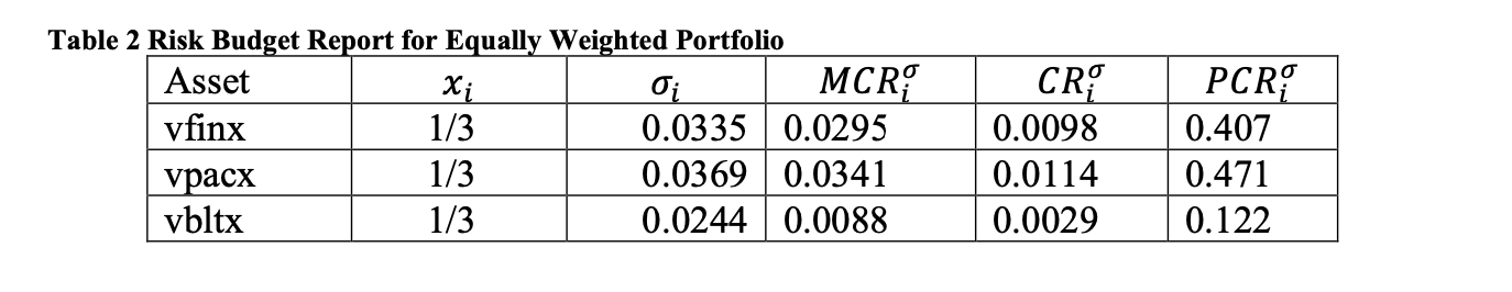1. Using the information from the risk report, what is the volatility (standard deviation) of the equally weighted portfolio?

2. In the equally weighted portfolio, do the assets have equal risk contributions? Which asset has the highest percent contribution to risk and which asset has the lowest percent contribution to risk?

3. Suppose the risk manager wants to reduce the portfolio volatility. For which assets should allocations be reduced, and for which assets should allocations be increased to achieve this goal?

14.9 Solutions to Selected Problems

w = c(1/3, 1/3, 1/3) sigma.mat = cov.mat[threeAssets, threeAssets]

sig.w = as.numeric(sqrt(t(w)%%sigma.mat%%w))

MCR.m = (sigma.mat%%w)/sig.w CR.m = wMCR.m PCR.m = CR.m/sig.w risk report: riskReport.pm = cbind(w, sd.vals[threeAssets], MCR.m, CR.m, PCR.m) colnames(riskReport.pm) = c(“Weight”, “Vol”, “MCR”, “CR”, “PCR”) riskReport.pm

compute beta: beta.m = PCR.m/w beta.m

compute rho: rho.m = MCR.m/sd.vals[threeAssets] rho.m

---

92. Two hedge funds, Bridgewater and AQR capital management have helped to make risk parity investing popular. ↩︎

93. It can be thought of as the population regression coefficient obtained by regressing the asset return, $R_{i},$on the portfolio return, $R_{p}(\mathbf{x}).$↩︎