9 Hypothesis Testing in the GWN Model

Updated: May 11, 2021

Copyright © Eric Zivot 2015, 2016, 2017, 2021

The core of statistical analysis involves estimation and inference. The previous chapters considered estimation of the GWN model parameters, and the computation of standard error estimates and confidence intervals. In this chapter we discuss issues of statistical inference within the GWN model. Statistical inference is about asking questions about a model and using statistical procedures to obtain answers to these questions with a given level of confidence. For example, we might find that our estimate of the monthly mean of an asset return is positive but due to large estimation error we might ask the question: is the true monthly mean return positive? As another example, we might find that a normal qq-plot of returns shows some evidence of non-normality and we ask the question: are returns normally distributed? As a third example, we might find that rolling estimates of the mean and volatility show some evidence of non-constant behavior and we might ask the question: are returns covariance stationary? Statistical hypothesis testing gives us a rigorous framework for answering such questions with a given level of confidence.

The R packages used in this chapter are IntroCompFinR, PerformanceAnalytics, tseries, and zoo. Make sure this packages are installed and loaded before replicating the examples.

1. Hypothesis Testing in the GWN Model
   1. Specification tests
      1. Normal distribution
         1. Tests for skewness and kurtosis
         2. JB test
         3. What to do if returns are not normally distributed?
      2. No autocorrelation A. individual and joint tests
      3. Constant parameters (covariance stationarity) A. Formal tests: testing same mean, volatility in sub-samples B. Informal diagnostics - standard error bands on rolling estimators
   2. Using Monte Carlo Simulation to Understand Hypothesis tests
      1. Size
      2. Power
   3. Using the bootstrap for hypothesis tests
      1. exploit duality between hypothesis tests and confidence intervals
2. Appendix: Distributions for test statistics
   1. Student’s t distribution
   2. Chi-square distribution

9.1 Review of General Principles

Classical hypothesis testing is discussed in almost all introductory textbooks on statistics, and the reader is assumed be familiar with the basic concepts.⁴⁶ In this section we provide a brief and concise review of the general principles of classical hypothesis testing. In the following sections we apply these principles to answer questions about the GWN model parameters and assumptions.

9.1.1 Steps for hypothesis testing

The main steps for conducting a classical hypothesis test are as follows:

1. Specify the hypotheses to be tested: \[ H_{0}:\textrm{null hypothesis vs. }H_{1}:\textrm{alternative hypothesis.} \] The null hypothesis is the maintained hypothesis (what is assumed to be true) and is the hypothesis to be tested against the data. The alternative hypothesis specifies what is assumed to be true if the null hypothesis is false. This can be specific or vague depending on the context.

2. Specify the significance level of the test: \[ \alpha=\textrm{significance level}=\Pr(\textrm{Reject }H_{0}|H_{0}\,\textrm{is true}). \] The significance level of a test specifies the probability of making a certain type of decision error: rejecting the null hypothesis when the null hypothesis is, in fact, true. In practice, the significance level \(\alpha\) is chosen to be a small number like \(0.01\) or \(0.05\).

3. Construct a test statistic, \(S\), from the observed data whose probability distribution is known when \(H_{0}\) is true.

4. Use the test statistic \(S\) to evaluate the data evidence regarding the validity of \(H_{0}\). Typically, if \(S\) is a big number then there is strong data evidence against \(H_{0}\) and \(H_{0}\) should be rejected; otherwise, there is not strong data evidence against \(H_{0}\) and \(H_{0}\) should not be rejected.

   • Decide to reject \(H_{0}\) at the specified significance level \(\alpha\) if the value of the test statistic \(S\) falls in the rejection region of the test. Usually, the rejection region for \(S\) is determined by a critical value \(cv_{\alpha}\) such that: \[\begin{eqnarray*} S & > & cv_{\alpha}\Rightarrow\mathrm{reject}\,H_{0},\\ S & \leq & cv_{\alpha}\Rightarrow\mathrm{do\,not\,reject}\,H_{0}. \end{eqnarray*}\] Smaller values of \(\alpha\) typically make \(cv_{\alpha}\) larger and require more data evidence (i.e., larger \(S\)) to reject \(H_{0}.\)

   • Alternatively, decide to reject \(H_{0}\) at the specified significance level \(\alpha\) if the p-value of the test statistic \(S\) is less than \(\alpha\). The p-value of the statistic \(S\) is defined as the significance level at which the test is just rejected.

9.1.2 Hypothesis tests and decisions

Hypothesis testing involves making a decision: reject \(H_{0}\) or do not reject \(H_{0}.\) Notice that if the data evidence strongly favors \(H_{0}\) then we say “we do not reject \(H_{0}\)” instead of “accept \(H_{0}\)”. We can rarely know the truth with absolute certainty with a finite amount of data so it is more appropriate to say “do not reject \(H_{0}\)” than to say “accept \(H_{0}\).”⁴⁷

Table 9.1: Decision table for hypothesis testing

		Reality
		\(H_{0}\) is true	\(H_{0}\) is false
Decision	Reject \(H_{0}\)	Type I error	No error
	Do not reject \(H_{0}\)	No error	Type II error

Table 9.2 shows the \(2\times2\) decision table associated with hypothesis testing. In reality there are two states of the world: either \(H_{0}\) is true or it is not.⁴⁸ There are two decisions to make: reject \(H_{0}\) or don’t reject \(H_{0}.\) If the decision corresponds with reality then the correct decision is made and there is no decision error. This occurs in the off-diagonal elements of the table. If the decision and reality disagree then there is a decision error. These errors are in the diagonal elements of the table. Type I error results when the decision to reject \(H_{0}\) occurs when, in fact, \(H_{0}\) is true. Type II error happens when the decision not to reject \(H_{0}\) occurs when \(H_{0}\) is false. To put these types of errors in context, consider a jury in a capital murder trial in the US.⁴⁹ In the US, a defendant is considered innocent until proven guilty. Here, the null hypothesis to be tested is: \[ H_{0}:\textrm{defendant is innocent}. \] The alternative is: \[ H_{1}:\textrm{defendant is guilty}. \]

There is a true state of the world here: the defendant is either innocent or guilty. The jury must decide what the state of the world is based on evidence presented to them. The decision table for the jury is shown in Table 9.2. Type I error occurs when the jury convicts an innocent defendant and puts that person on “death row”. Clearly, this is a terrible mistake. To avoid this type of mistake the jury should have a very small (close to zero) significance level for evaluating evidence so that Type I error very rarely occurs. This is why typical jury instructions are to convict only if evidence of guilt is presented beyond reasonable doubt. Type II error happens when the jury does not convict (acquits) a guilty defendant and sets that person free. This is also a terrible mistake, but perhaps it is not as terrible as convicting the innocent person. Notice that there is a conflict between Type I error and Type II error. In order to completely eliminate Type I error, you can never reject \(H_{0}\). That is, to avoid ever sending innocent people to “death row” you must never convict anyone. But if you never convict anyone then you never convict guilty people either and this increases the occurrences of Type II errors.

9.1.3 Significance level and power

The significance level of a test is the probability of Type I error: \[ \alpha=\Pr(\textrm{Type I error})=\Pr(\textrm{Reject}\,H_{0}|H_{0}\,\textrm{is true}). \] The power of a test is one minus the probability of Type II error: \[ \pi=1-\Pr(\textrm{Type II error})=\Pr(\textrm{Reject }H_{0}|H_{0}\,\textrm{is false}). \] In classical hypothesis tests, the goal is to construct a test that has a small significance level (\(\alpha\) close to zero) that you can control and has high power (\(\pi\) close to one). That is, a good test is one that has a small and controllable probability of rejecting the null when it is true and, at the same time, has a very high probability of rejecting the null when it is false. In general, an optimal test is one that has the highest possible power for a given significance level. In the jury example, an optimal test would be the one in which the jury has the highest probability of convicting a guilty defendant while at the same time has a very low probability of convicting an innocent defendant. A difficult problem indeed!

Table 9.2: Decision table for jury on capital murder trial

		Reality
		Defendant is innocent	Defendant is guilty
Decision	Convict	Type I error	No error
	Acquit	No error	Type II error

9.2 Hypothesis Testing in the GWN Model

In this section, we discuss hypothesis testing in the context of the GWN model for asset returns:

\[\begin{align} R_{it} & =\mu_{i}+\varepsilon_{it},\,i=1\ldots,N;\,t=1,\ldots,T\tag{9.1}\\ \{\varepsilon_{it}\}_{t=1}^{T} & \sim\mathrm{GWN}(0,\sigma_{i}^{2}),\nonumber \\ \mathrm{cov}(\varepsilon_{it},\varepsilon_{js}) & =\left\{\begin{array}{c} \sigma_{ij}\\ 0 \end{array}\right.\begin{array}{c} t=s\\ t\neq s \end{array}.\nonumber \end{align}\]

In (9.1), \(R_{it}\) is the monthly return (continuously compounded or simple) on asset \(i\) in month \(t\). Define \(\mathbf{R}_{t}=(R_{1t},\ldots,R_{Nt})^{\prime}\). The GWN model in matrix form is:

\[\begin{align} \mathbf{R}_{t}=\mu+\varepsilon_{t},\tag{9.2}\\ \varepsilon_{t}\sim\mathrm{iid}~N(\mathbf{0},\Sigma).\nonumber \end{align}\]

We consider two types of hypothesis tests: (1) tests for model coefficients or functions of model coefficients; and (2) tests for model assumptions.⁵⁰ These tests can be specified for the GWN model for a single asset using (9.1), or they can be specified for the GWN model for all assets using (9.2).

9.2.1 Coefficient tests

Here, we assume that the GWM is the true model for our observed return data and we are interested in asking questions about the parameters of the model. The most common tests for model coefficients and functions of model coefficients for a single asset are tests for a specific value. Some typical hypotheses to be tested are:

\[\begin{align*} H_{0} & :\mu_{i}=\mu_{i}^{0}\text{ vs. }H_{1}:\mu_{i}\neq\mu_{i}^{0},\\ H_{0} & :\sigma_{i}=\sigma_{i}^{0}\text{ vs. }H_{1}:\sigma_{i}\neq\sigma_{i}^{0},\\ H_{0} & :\rho_{ij}=\rho_{ij}^{0}\text{ vs. }H_{1}:\rho_{ij}\neq\rho_{ij}^{0}, \\ H_{0} & :\mathrm{SR}_{i}=\mathrm{SR}_{i}^{0}\text{ vs. }H_{1}:\mathrm{SR}_{i}\neq\mathrm{SR}_{i}^{0}, \end{align*}\]

where \(\mathrm{SR}_{i} = \frac{\mu_i - r_f}{\sigma_i}\) is the Sharpe ratio of asset \(i\) and \(r_f\) is the risk-free rate of interest. A hypothesis about the Sharpe ratio is a hypothesis about the ratio of two GWN model parameters. In the above hypotheses, the alternative hypotheses are two-sided. That is, under \(H_{1}\) the model parameters are either larger or smaller than what is specified under \(H_{0}\).

Also common are tests for specific sign. For example:

\[\begin{align*} H_{0} & :\mu_{i}=0\text{ vs. }H_{1}:\mu_{i}>0\text{ or }H_{1}:\mu_{i}<0,\\ H_{0} & :\rho_{ij}=0\text{ vs. }H_{1}:\rho_{ij}>0\text{ or }H_{1}:\rho_{ij}<0, \\ H_{0} & :\mathrm{SR}_{i}=0\text{ vs. }H_{1}:\mathrm{SR}_{i}>0\text{ or }H_{1}:\mathrm{SR}_{i}<0, \end{align*}\]

Here, the alternative hypotheses are one-sided. That is, under \(H_{1}\) the model parameter is either greater than zero or less than zero.

Sometimes we are interested in testing hypotheses about the relationship between model coefficients for two or more assets. For example:

\[\begin{align*} H_{0} & :\mu_{1}=\mu_{2}\,\textrm{vs. } H_{1}:\mu_{1}\neq\mu_{2}, \\ H_{0} & :\mathrm{SR}_{1}=\mathrm{SR}_{2}\,\textrm{vs. } H_{1}:\mathrm{SR}_{1}\neq\ \mathrm{SR}_{2}. \end{align*}\]

It is often convenient to re-express these hypotheses in terms of differences of coefficients under the null and alternative hypotheses:

\[\begin{align*} H_{0} & :\mu_{1}-\mu_{2}=0 \,\textrm{vs. } H_{1}:\mu_{1}-\mu_{2} \neq 0, \\ H_{0} & :\mathrm{SR}_{1}-\mathrm{SR}_{2}=0 \,\textrm{vs. } H_{1}:\mathrm{SR}_{1}- \mathrm{SR}_{2} \neq 0. \end{align*}\]

9.2.2 Model specification tests

In the GWN model (9.1), asset returns are assumed to be normally distributed. The hypotheses to be tested for this assumption are:

\[\begin{align*} H_{0}: & R_{it}\sim N(\mu_{i},\sigma_{i}^{2})\,\textrm{vs. }H_{1}:R_{it}\sim\textrm{ not normal.} \end{align*}\]

Notice that the distribution of \(R_{t}\) under \(H_{1}\) is not specified (e.g., Student’s t with 5 degrees of freedom).

In addition, it is assumed that asset returns are uncorrelated over time. One can test the hypothesis that each autocorrelation (up to some maximum lag \(J\)) is zero:

\[\begin{align*} H_{0} & :\rho_{j}=\mathrm{cor}(r_{it},r_{i,t-j})=0\text{, }j=1,\ldots,J\,\mathrm{vs}.\\ H_{1} & :\rho_{j}=\mathrm{cor}(r_{it},r_{i,t-j})\neq0, \end{align*}\]

or one can test the joint hypothesis that all autocorrelation coefficients (up to some maximum lag \(J\)) are zero:

\[\begin{eqnarray*} H_{0}:\rho_{1} & = & \rho_{2}=\cdots=\rho_{J}=0\,vs.\\ H_{1}:\rho_{j} & \neq & 0\,\textrm{for some }j\leq J \end{eqnarray*}\]

Lastly, it is assumed that asset returns are covariance stationary. This assumption implies that all model parameters are constant over time. The hypotheses of interest are then:

\[\begin{align*} H_{0} & :\mu_{i},\sigma_{i}\text{ and }\rho_{ij}\text{ are constant over entire sample, vs.}\\ H_{1} & :\mu_{i}\text{ }\sigma_{i}\text{ or }\rho_{ij}\text{ changes in some sub-sample.} \end{align*}\]

The following sections describe test statistics for the above listed hypotheses.

9.2.3 Data for hypothesis testing examples

The examples in this chapter use the monthly continuously compounded returns on Microsoft, Starbucks and the S&P 500 index over the period January 1998 through May 2012 created using:

data(msftDailyPrices, sbuxDailyPrices, sp500DailyPrices) 
gwnDailyPrices = merge(msftDailyPrices, sbuxDailyPrices, sp500DailyPrices)
gwnMonthlyPrices = to.monthly(gwnDailyPrices, OHLC=FALSE) 

## Warning in to.period(x, "months", indexAt = indexAt, name =
## name, ...): missing values removed from data

smpl = "1998-01::2012-05" 
gwnMonthlyPrices = gwnMonthlyPrices[smpl] 
gwnMonthlyRetC = na.omit(Return.calculate(gwnMonthlyPrices, method="log"))

The monthly continuously compounded returns, with a common y-axis, are illustrated in Figure 9.1 created using:

plot(gwnMonthlyRetC, multi.panel=TRUE, main="",
     col="blue", lwd=2, yaxis.same=TRUE,
     major.ticks="years", grid.ticks.on="years")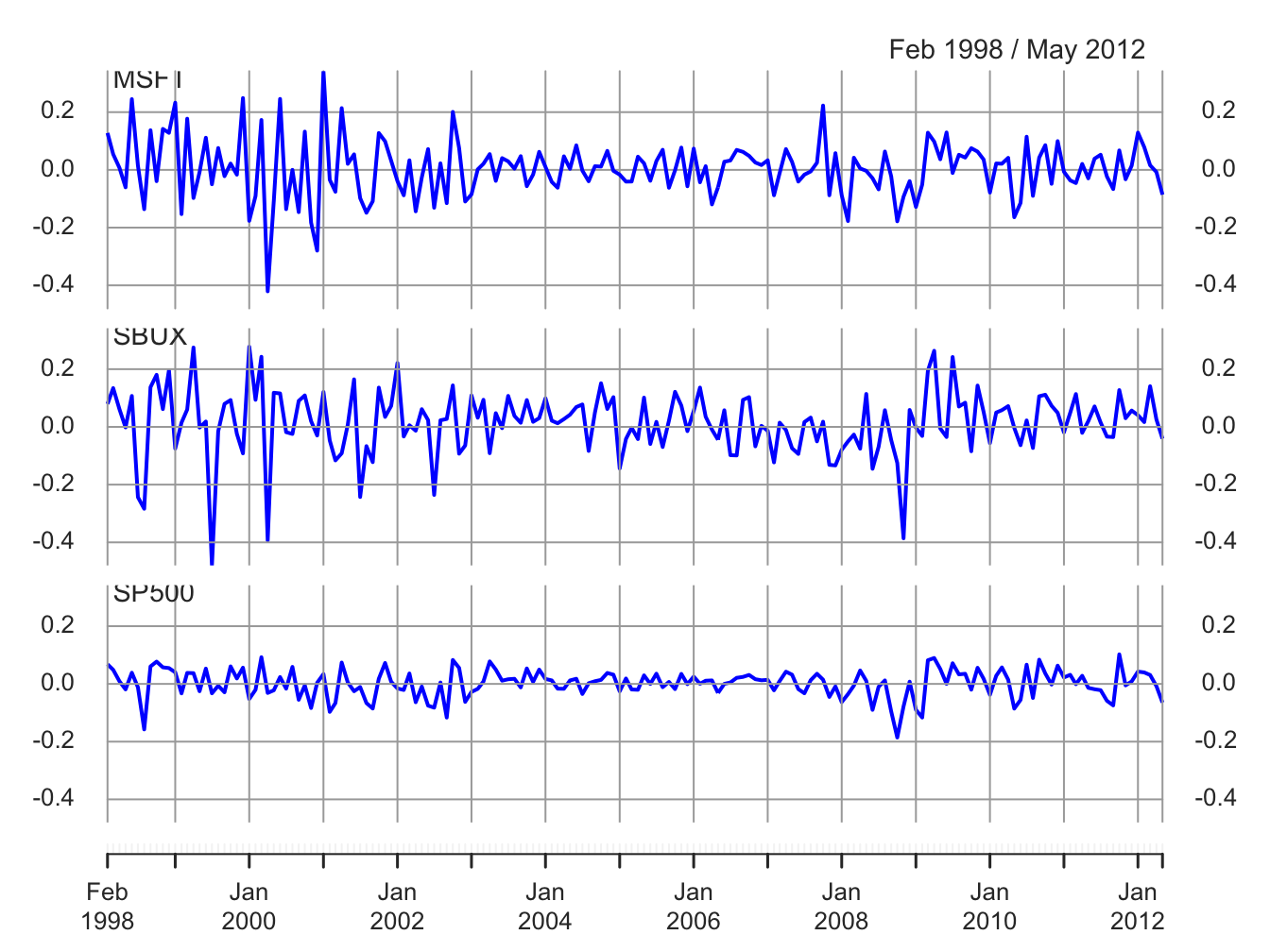

Figure 9.1: Monthly cc returns on Microsoft, Starbucks and the S&P 500 Index.

9.3 Tests for Individual Parameters: t-tests and z-scores

In this section, we present test statistics for testing hypotheses that certain model coefficients equal specific values. In some cases, we can derive exact tests. For an exact test, the pdf of the test statistic assuming the null hypothesis is true is known exactly for a finite sample size \(T\). More generally, however, we rely on asymptotic tests. For an asymptotic test, the pdf of the test statistic assuming the null hypothesis is true is not known exactly for a finite sample size \(T\), but can be approximated by a known pdf. The approximation is justified by the Central Limit Theorem (CLT) and the approximation becomes exact as the sample size becomes infinitely large.

9.3.1 Exact tests under normality of data

In the GWN model (9.1), consider testing the hypothesis that the mean return, \(\mu_{i}\), is equal to a specific value \(\mu_{i}^{0}\):

\[\begin{equation} H_{0}:\mu_{i}=\mu_{i}^{0}.\tag{9.3} \end{equation}\]

For example, an investment analyst may have provided an expected return forecast of \(\mu_{i}^{0}\) and we would like to see if past data was consistent with such a forecast.

The alternative hypothesis can be either two-sided or one-sided. The two-sided alternative is: \[\begin{equation} H_{1}:\mu_{i}\neq\mu_{i}^{0}.\tag{9.4} \end{equation}\] Two-sided alternatives are used when we don’t care about the sign of \(\mu_{i}-\mu_{i}^{0}\) under the alternative. With one-sided alternatives, we care about the sign of \(\mu_{i}-\mu_{i}^{0}\) under the alternative: \[\begin{equation} H_{1}:\mu_{i}>\mu_{i}^{0}\,\textrm{ or }\,H_{1}:\mu_{i}<\mu_{i}^{0}.\tag{9.5} \end{equation}\] How do we come up with a test statistic \(S\) for testing (9.3) against (9.4) or (9.5)? We generally use two criteria: (1) we know the pdf of \(S\) assuming (9.3) is true; and (2) the value of \(S\) should be big if the alternative hypotheses (9.4) or (9.5) are true.

9.3.1.1 Two-sided test

To simplify matters, let’s assume that the value of \(\sigma_{i}\) in (9.1) is known and does not need to be estimated. This assumption is unrealistic and will be relaxed later. Consider testing (9.3) against the two-sided alternative (9.4) using a 5% significance level. Two-sided alternatives are typically more commonly used than one-sided alternatives. Let \(\{R_{t}\}_{t=1}^{T}\) denote a random sample from the GWN model. We estimate \(\mu_{i}\) using the sample mean:

\[\begin{equation} \hat{\mu}_{i}=\frac{1}{T}\sum_{t=1}^{T}R_{it}.\tag{9.6} \end{equation}\]

Under the null hypothesis (9.3), it is assumed that \(\mu_{i}=\mu_{i}^{0}\). Hence, if the null hypothesis is true then \(\hat{\mu}_{i}\) computed from data should be close to \(\mu_{i}^{0}\). If \(\hat{\mu}_{i}\) is far from \(\mu_{i}^{0}\) (either above or below \(\mu_{i}^{0}\)) then this evidence casts doubt on the validity of the null hypothesis. Now, there is estimation error in (9.6) which is measured by:

\[\begin{equation} \mathrm{se}(\hat{\mu}_{i})=\frac{\sigma_{i}}{\sqrt{T}}.\tag{9.7} \end{equation}\]

Because we assume \(\sigma_{i}\) is known, we also know \(\mathrm{se}(\hat{\mu}_{i})\). Because of estimation error, we don’t expect \(\hat{\mu}_{i}\) to equal \(\mu_{i}^{0}\) even if the null hypothesis (9.3) is true. How far from \(\mu_{i}^{0}\) can \(\hat{\mu}_{i}\) be if the null hypothesis is true? To answer this question, recall from Chapter 7 that the exact (finite sample) pdf of \(\hat{\mu}_{i}\) is the normal distribution:

\[\begin{equation} \hat{\mu}_{i}\sim N(\mu_{i},\mathrm{se}(\hat{\mu}_{i})^{2})=N\left(\mu_{i},\frac{\sigma_{i}^{2}}{T}\right).\tag{9.8} \end{equation}\]

Under the null hypothesis (9.3), the normal distribution for \(\hat{\mu}_{i}\) is centered at \(\mu_{i}^{0}\):

\[\begin{equation} \hat{\mu}_{i}\sim N(\mu_{i}^{0},\mathrm{se}(\hat{\mu}_{i})^{2})=N\left(\mu_{i}^{0},\frac{\sigma_{i}^{2}}{T}\right).\tag{9.9} \end{equation}\]

From properties of the normal distribution we have:

\[\begin{equation} \Pr\left(\mu_{i}^{0}-1.96\times\mathrm{se}(\hat{\mu}_{i})\leq\hat{\mu}_{i}\leq\mu_{i}^{0}+1.96\times\mathrm{se}(\hat{\mu}_{i})\right)=0.95.\tag{9.10} \end{equation}\]

Hence, if the null hypothesis (9.3) is true we only expect to see \(\hat{\mu}_{i}\) more than \(1.96\) values of \(\mathrm{se}(\hat{\mu}_{i})\) away from \(\mu_{i}^{0}\) with probability 0.05.⁵¹ Therefore, it makes intuitive sense to base a test statistic for testing (9.3) on a measure of distance between \(\hat{\mu}_{i}\) and \(\mu_{i}^{0}\) relative to \(\mathrm{se}(\hat{\mu}_{i})\). Such a statistic is the z-score:

\[\begin{equation} z_{\mu=\mu^{0}}=\frac{\hat{\mu}_{i}-\mu_{i}^{0}}{\mathrm{se}(\hat{\mu}_{i})}=\frac{\hat{\mu}_{i}-\mu_{i}^{0}}{\sigma/\sqrt{T}}.\tag{9.11} \end{equation}\]

Assuming the null hypothesis (9.3) is true, from (9.9) it follows that: \[ z_{\mu=\mu^{0}}\sim N(0,1). \]

The intuition for using the z-score (9.11) to test (9.3) is straightforward. If \(z_{\mu=\mu^{0}}\approx0\) then \(\hat{\mu}_{i}\approx\mu_{i}^{0}\) and (9.3) should not be rejected. In contrast, if \(z_{\mu=\mu^{0}}>1.96\) or \(z_{\mu=\mu^{0}}<-1.96\) then \(\hat{\mu}_{i}\) is more than \(1.96\) values of \(\mathrm{se}(\hat{\mu}_{i})\) away from \(\mu_{i}^{0}\). From (9.10), this is very unlikely (less than 5% probability) if (9.3) is true. In this case, there is strong data evidence against (9.3) and we should reject it. Notice that the condition \(z_{\mu=\mu^{0}}>1.96\textrm{ or }z_{\mu=\mu^{0}}<-1.96\) can be simplified as the condition \(\left|z_{\mu=\mu^{0}}\right|>1.96\). When \(\left|z_{\mu=\mu^{0}}\right|\) is big, larger than 1.96, we have data evidence against (9.3). Using the value \(1.96\) to determine the rejection region for the test ensures that the significance level (probability of Type I error) of the test is exactly 5%:

\[\begin{align*} \Pr(\textrm{Reject } H_{0}|H_{0}\,\textrm{is true}) &= \Pr(S>1.96|\mu_{i}=\mu_{i}^{0}) \\ &=\Pr\left(\left|z_{\mu=\mu^{0}}\right|>1.96|\mu_{i}=\mu_{i}^{0}\right)=.05 \end{align*}\]

Hence, our formal test statistic for testing (9.3) against (9.4) is

\[\begin{equation} S=\left|z_{\mu=\mu^{0}}\right|. \tag{9.12} \end{equation}\]

The 5% critical value is \(cv_{.05}=1.96\), and we reject (9.3) at the 5% significance level if \(S>1.96\).

In summary, the steps for using \(S=\left|z_{\mu=\mu^{0}}\right|\) to test the (9.3) against (9.4) are:

1. Set the significance level \(\alpha=\Pr(\textrm{Reject } H_{0}|H_{0}\,\textrm{is true})\) and determine the critical value \(cv_{\alpha}\) such that \(\Pr(S>cv_{\alpha})=\alpha\). Now,

\[\begin{align*} \Pr(S>cv_{\alpha}) &= \Pr\left(\left|z_{\mu=\mu^{0}}\right|>cv_{\alpha}\right) \\ &= \Pr\left(z_{\mu=\mu^{0}}>cv_{\alpha}\right)+\Pr\left(z_{\mu=\mu^{0}}<-cv_{\alpha}\right)=\alpha \end{align*}\]

which implies that \(cv_{\alpha}=-q_{\alpha/2}^{Z}=q_{1-\alpha/2}^{Z}\), where \(q_{\alpha/2}^{Z}\) denotes the \(\frac{\alpha}{2}-\)quantile of \(Z\sim N(0,1)\). For example, if \(\alpha=.05\) then \(cv_{.05}=-q_{.025}^{Z}=1.96.\)

2. Reject (9.3) at the \(\alpha\times100\%\) significance level if \(S>cv_{\alpha}\). For example, if \(\alpha=.05\) then reject (9.3) at the 5% level if \(S>1.96\).

3. Equivalently, reject (9.3) at the \(\alpha\times100\%\) significance level if the p-value for \(S\) is less than \(\alpha\). Here, the p-value is defined as the significance level at which the test is just rejected. Let \(Z\sim N(0,1)\). The p-value is computed as: \[\begin{eqnarray} \textrm{p-value} & = & \Pr(|Z|>S)=\Pr(Z>S)+\Pr(Z<-S)\\ & = & 2\times \Pr(Z>S)=2\times(1-\Pr(Z<S)) \tag{9.13}. \end{eqnarray}\]

Example 9.1 (Testing hypothesis with the z-score using simulated data: two-sided tests)

Assume returns follow the GWN model

\[\begin{eqnarray*} R_{t} & = & 0.05+\epsilon_{t},\,t=1,\ldots60,\\ \epsilon_{t} & \sim & GWN(0,0.10). \end{eqnarray*}\]

and we are interested in testing the following hypotheses \[\begin{align*} H_{0}:\mu=0.05\,\,vs.\,\,H_{1}:\mu\neq.05 \\ H_{0}:\mu=0.06\,\,vs.\,\,H_{1}:\mu\neq.06 \\ H_{0}:\mu=0.10\,\,vs.\,\,H_{1}:\mu\neq.10 \\ \end{align*}\]

using the test statistic (9.12) with a 5% significance level. The 5% critical value is \(cv_{.05}=1.96\). One hypothetical sample from the hypothesized model is simulated using:

set.seed(123)
n.obs = 60
mu = 0.05
sigma = 0.10
ret.sim = mu + rnorm(n.obs, sd = sigma)

The estimate of \(\mu\) and the value of \(\mathrm{se}(\hat{\mu})\) are:

muhat = mean(ret.sim)
se.muhat = sigma/sqrt(n.obs)
c(muhat, se.muhat)

## [1] 0.0566 0.0129

The test statistic (9.12) for testing \(H_0:\mu=0.05\) computed from this sample is:

z.score.05 = (muhat - 0.05)/se.muhat
S = abs(z.score.05)
S

## [1] 0.508

The z-score tells us that the estimated mean, \(\hat{\mu}=0.0566\), is 0.58 values of \(\mathrm{se}(\hat{\mu})\) away from the hypothesized value \(\mu^0=0.05\). This evidence does not contradict \(H_0:\mu=0.05\). Since \(S=0.508 < 1.96\), we do not reject \(H_0:\mu=0.05\) at the 5% significance level. The p-value of the test using (9.13) is:

p.value = 2*(1 - pnorm(S))
p.value

## [1] 0.611

Here, the p-value of 0.611 is less than the significance level \(\alpha = 0.05\) so we do not reject the null at the 5% significance level. The p-value tells us that we would reject \(H0:\mu=0.05\) at the 61.1% significance level.

The z-score information for testing \(H_0:\mu=0.06\) is:

z.score.06 = (muhat - 0.06)/se.muhat
S = abs(z.score.06)
S

## [1] 0.266

Here, the z-score indicates that \(\hat{\mu}=0.0566\) is just 0.266 values of \(\mathrm{se}(\hat{\mu})\) away from the hypothesized value \(\mu^0=0.06\). This evidence also does not contradict \(H_0:\mu=0.06\). Since \(S=0.226 < 1.96\), we do not reject \(H_0:\mu=0.06\) at the 5% significance level. The p-value of the test is:

p.value = 2*(1 - pnorm(S))
p.value

## [1] 0.79

The large p-value shows that there is insufficient data to reject \(H_0:\mu=0.06\).

Last, the z-score information for testing \(H_0:\mu=0.10\) is:

z.score.10 = (muhat - 0.10)/se.muhat
S = abs(z.score.10)
S

## [1] 3.36

Now, the z-score indicates that \(\hat{\mu}=0.0566\) is 3.36 values of \(\mathrm{se}(\hat{\mu})\) away from the hypothesized value \(\mu^0=0.10\). This evidence is not in support of \(H_0:\mu=0.10\). Since \(S=3.36 > 1.96\), we reject \(H_0:\mu=0.06\) at the 5% significance level. The p-value of the test is:

p.value = 2*(1 - pnorm(S))
p.value

## [1] 0.000766

Here, the p-value is much less 5% supporting the rejection of \(H_0:\mu=0.06\).

\(\blacksquare\)

9.3.1.2 One-sided test

Here, we consider testing the null (9.3) against the one-sided alternative (9.5). For expositional purposes, consider \(H_{1}:\mu_{i} > \mu_{i}^{0}\). This alternative can be equivalently represented as \(H_{1}:\mu_{i} - \mu_{i}^{0} > 0\). That is, under the alternative hypothesis the sign of the difference \(\mu_{i} - \mu_{i}^{0}\) is positive. This is why a test against a one-sided alternative is sometimes called a test for sign. As in the previous sub-section, assume that \(\sigma_i\) is known and let the significance level be \(5\%\).

The natural test statistic is the z-score (9.11): \[ S = z_{\mu = \mu^0}. \]

The intuition is straightforward. If \(z_{\mu=\mu^0} \approx 0\) then \(\hat{\mu}_i \approx \mu_i^0\) and the null should not be rejected. However, if the one-sided alternative is true then we would expect to see \(\hat{\mu}_i > \mu_i^0\) and \(z_{\mu=\mu^0} > 0\). How big \(z_{\mu=\mu^0}\) needs to be for us to reject the null depends on the significance level. Since under the null \(z_{\mu=\mu^0} \sim N(0,1) = Z\), with a \(5\%\) significance level

\[ \Pr(\text{Reject } H_0 | H_0 \text{ is true}) = \Pr(z_{\mu=\mu^0} > 1.645) = \Pr(Z > 1.645) = 0.05. \] Hence, our \(5\%\) one-sided critical value is \(cv_{.05}=q_{.95}^Z = 1.645\), and we reject the null at the \(5\%\) significance level if \(z_{\mu=\mu^0} >1.645\).

In general, the steps for using \(z_{\mu=\mu^0}\) to test (9.3) against the one-sided alternative \(H_{1}:\mu_{i} > \mu_{i}^{0}\) are:

1. Set the significance level \(\alpha=\Pr(\textrm{Reject } H_{0}|H_{0}\,\textrm{is true})\) and determine the critical value \(cv_{\alpha}\) such that \(\Pr(z_{\mu=\mu^0}>cv_{\alpha})=\alpha\). Since under the null \(z_{\mu=\mu^0} \sim N(0,1) = Z\), \(cv_{\alpha} = q_{1-\alpha}^Z\).

2. Reject the null hypothesis (9.3) at the \(\alpha \times 100\%\) significance level if \(z_{\mu=\mu^0} > cv_{\alpha}\).

3. Equivalently, reject (9.3) at the \(\alpha \times 100\%\) significance level if the one-sided p-value is less than \(\alpha\), where

\[ \text{p-value} = \Pr(Z > z_{\mu=\mu^0}) = 1 - \Pr(Z \le z_{\mu=\mu^0}) \]

Example 9.2 (Testing hypothesis with the z-score using simulated data: one-sided tests)

Here, we use the simulated GWN return data from the previous example to test (9.3) against the one-sided alternative \(H_{1}:\mu_{i} > \mu_{i}^{0}\) using a 5% significance level.

The z-scores and one-sided p-values for testing \(H_0:\mu=0.05\), \(H_0:\mu=0.06\), and \(H_0:\mu=0.10\), computed from the simulated sample are:

z.score.05 = (muhat - 0.05)/se.muhat
p.value.05 = 1 - pnorm(z.score.05)
z.score.06 = (muhat - 0.06)/se.muhat
p.value.06 = 1 - pnorm(z.score.06)
z.score.10 = (muhat - 0.10)/se.muhat
p.value.10 = 1 - pnorm(z.score.10)
ans = rbind(c(z.score.05, p.value.05),
            c(z.score.06, p.value.06),
            c(z.score.10, p.value.10))
colnames(ans) = c("Z-score", "P-value")
rownames(ans) = c("H0:mu=0.05", "H0:mu=0.06","H0:mu=0.10")
ans

##            Z-score P-value
## H0:mu=0.05   0.508   0.306
## H0:mu=0.06  -0.266   0.605
## H0:mu=0.10  -3.365   1.000

Here, we do not reject any of the null hypotheses in favor of the one-sided alternative at the 5% significance level.

9.3.2 Exact tests with \(\sigma\) unknown

In practice, \(\sigma^2\) is unknown and is estimated with \(\hat{\sigma}\), and so the exact tests described above are not feasible. Fortunately, an exact test is still available. Instead of using the z-score (9.11), we use the t-ratio (or t-score)

\[\begin{equation} t_{\mu=\mu^0}=\frac{\hat{\mu}_{i}-\mu_{i}^0}{\widehat{\mathrm{se}}(\hat{\mu}_{i})}=\frac{\hat{\mu}_{i}-\mu_{i}^0}{\hat{\sigma}/\sqrt{T}}.\tag{9.14} \end{equation}\]

Assuming the null hypothesis (9.3) is true, Proposition 7.7 tells us that (9.14) is distributed Student’s t with \(T-1\) degrees of freedom and is denoted by the random variable \(t_{T-1}\). The steps for using the z-score and the t-ratio are the same for evaluating (9.3), but now we use critical values and p-values from \(t_{T-1}\). Our test statistic for the two-sided alternative \(H_0:\mu_i \ne \mu_i^0\) is: \[\begin{equation} S = \left|t_{\mu=\mu^{0}}\right|, \tag{9.15} \end{equation}\]

and our test statistic for the one-sided alternative \(H_0:\mu_i > \mu_i^0\) is

\[\begin{equation} S = t_{\mu=\mu^{0}}, \tag{9.16} \end{equation}\]

Our critical values are determined from the quantiles of the Student’s t with \(T-1\) degrees of freedom, \(t_{T-1}(1-\alpha/2)\). For example, if \(\alpha=0.05\) and \(T-1=60\) then the two-sided critical value is \(cv_{.05} = t_{60}(0.975)=2\) (which can be verified using the R function qt()). The two-sided p-value is computed as:

\[\begin{eqnarray*} \textrm{p-value} & = & \Pr(|t_{T-1}|>S)=\Pr(t_{T-1}>S)+\Pr(t_{T-1}<-S)\\ & = & 2\times \Pr(t_{T-1}>S)=2\times(1-\Pr(t_{T-1}<S)). \end{eqnarray*}\]

The one-sided critical value is \(cv_{.05} = t_{60}(0.95)=1.67\), and the one-sided p-value is computed as:

\[ \text{p-value} = \Pr(t_{T-1} > S) = 1 - \Pr(t_{T-1} \le S). \]

As the sample size gets larger \(\hat{\sigma}_{i}\) gets closer to \(\sigma_{i}\) and the Student’s t distribution gets closer to the normal distribution. Decisions using the t-ratio and the z-score are almost the same for \(T \ge 60\).

Example 9.3 (Testing hypothesis with the t-ratio using simulated data)

We repeat the hypothesis testing from the previous example this time use the t-ratio (9.14) instead of the z-score. Using \(T-1=59\) the 5% critical value for the two-sided test is

qt(0.975, df=59)

## [1] 2

To compute the t-ratios we first estimate \(\mathrm{se}(\hat{\mu})\):

sigmahat = sd(ret.sim)
sehat.muhat = sigmahat/sqrt(n.obs)
c(sehat.muhat, se.muhat)

## [1] 0.0118 0.0129

Here, \(\widehat{\mathrm{se}}(\hat{\mu}) = 0.0118 < 0.0129 = \mathrm{se}(\hat{\mu})\) and so the t-ratios will be slightly larger than the z-scores. The t-ratios and test statistics for the three hypotheses are:

t.ratio.05 = (muhat - 0.05)/sehat.muhat
t.ratio.06 = (muhat - 0.06)/sehat.muhat
t.ratio.10 = (muhat - 0.10)/sehat.muhat
S.05 = abs(t.ratio.05)
S.06 = abs(t.ratio.06)
S.10 = abs(t.ratio.10)
ans = c(S.05, S.06, S.10)
names(ans) = c("S.05", "S.06", "S.07")
ans

##  S.05  S.06  S.07 
## 0.558 0.293 3.696

As expected the test statistics computed from the t-ratios are slightly larger than the tests computed from the z-scores. The first two statistics are less than 2, and the third statistic is bigger than 2 and so we reach the same decisions as before. The p-values of the three tests are:

S.vals = c(S.05, S.06, S.10)
p.values = 2*(1 - pt(S.vals, df=59))
p.values

## [1] 0.578747 0.770895 0.000482

Here, the p-values computed from \(t_{59}\) are very similar to those computed from \(Z\sim N(0,1)\).

\(\blacksquare\)

We can derive an exact test for testing hypothesis about the value of \(\mu_{i}\) based on the z-score or the t-ratio, but we cannot derive exact tests for the values of \(\sigma_{i}\) or for the values of \(\rho_{ij}\) based on z-scores. Exact tests for these parameters are much more complicated. While t-ratios for the values of \(\sigma_{i}\) or for the values of \(\rho_{ij}\) do not have exact t-distributions in finite samples, as the sample size gets large the distributions of the t-ratios get closer and closer to the normal distribution due to the CLT. This motivates the use of so-called asymptotic z-scores discussed in the next sub-section.

9.3.3 Z-scores under asymptotic normality of estimators

Let \(\hat{\theta}\) denote an estimator for \(\theta\). Here, we allow \(\theta\) to be a GWN model parameter or a function of GWN model parameters. For example, in the GWN model \(\theta\) could be \(\mu_{i}\), \(\sigma_{i},\), \(\rho_{ij}\), \(q_{\alpha}^R\), \(\mathrm{VaR}_{\alpha}\) or \(\mathrm{SR}_i\). As we have seen, the CLT (and the delta method if needed) justifies the asymptotic normal distribution:

\[\begin{equation} \hat{\theta}\sim N(\theta,\widehat{\mathrm{se}}(\hat{\theta})^{2}),\tag{9.17} \end{equation}\]

for large enough sample size \(T\), where \(\widehat{\mathrm{se}}(\hat{\theta})\) is the estimated standard error for \(\hat{\theta}\). Consider testing:

\[\begin{equation} H_{0}:\theta=\theta_{0}\text{ vs. }H_{1}:\theta\neq\theta_{0}.\tag{9.18} \end{equation}\]

Under \(H_{0},\) the asymptotic normality result (9.17) implies that the z-score for testing (9.18) has a standard normal distribution for large enough sample size \(T\):

\[\begin{equation} z_{\theta=\theta_{0}}=\frac{\hat{\theta}-\theta_{0}}{\widehat{\mathrm{se}}(\hat{\theta})}\sim N(0,1)=Z.\tag{9.19} \end{equation}\]

The intuition for using the z-score (9.19) is straightforward. If \(z_{\theta=\theta_{0}}\approx0\) then \(\hat{\theta}\approx\theta_{0},\) and \(H_{0}:\theta=\theta_{0}\) should not be rejected. On the other hand, if \(|z_{\theta=\theta_{0}}|>2\), say, then \(\hat{\theta}\) is more than \(2\) values of \(\widehat{\mathrm{se}}(\hat{\theta})\) away from \(\theta_{0}.\) This is very unlikely if \(\theta=\theta_{0}\) because \(\hat{\theta}\sim N(\theta_{0},\mathrm{\widehat{se}}(\hat{\theta})^{2}),\) so \(H_{0}:\theta\neq\theta_{0}\) should be rejected. Therefore, the test statistic for testing (9.19) is \(S = |z_{\theta=\theta_{0}}|\).

The steps for using the z-score (9.19) with its critical value to test the hypotheses (9.18) are:

1. Set the significance level \(\alpha\) of the test and determine the two-sided critical value \(cv_{\alpha/2}\). Using (9.17), the critical value, \(cv_{\alpha/2},\) is determined using: \[\begin{align*} \Pr(|Z| & \geq cv_{\alpha/2})=\alpha\\ & \Rightarrow cv_{\alpha/2}=-q_{\alpha/2}^{Z}=q_{1-\alpha/2}^{Z}, \end{align*}\] where \(q_{\alpha/2}^{Z}\) denotes the \(\frac{\alpha}{2}-\)quantile of \(N(0,1)\). A commonly used significance level is \(\alpha=0.05\) and the corresponding critical value is \(cv_{.025}=-q_{.025}^{Z}=q_{.975}^{Z}=1.96\approx2\).

2. Reject (9.18) at the \(100\times\alpha\)% significance level if: \[ S = |z_{\theta=\theta_{0}}|=\left\vert \frac{\hat{\theta}-\theta^{0}}{\widehat{\mathrm{se}}(\hat{\theta})}\right\vert >cv_{\alpha/2}. \] If the significance level is \(\alpha=0.05\), then reject (9.18) at the 5% level using the rule-of-thumb: \[ S=|z_{\theta=\theta_{0}}|>2. \]

The steps for using the z-score (9.19) with its p-value to test the hypotheses (9.18) are:

1. Determine the two-sided p-value. The p-value of the two-sided test is the significance level at which the test is just rejected. From (9.17), the two-sided p-value is defined by \[\begin{equation} \textrm{p-value}=\Pr\left(|Z|>|z_{\theta=\theta_{0}}|\right)=2\times(1-\Pr\left(Z\leq|z_{\theta=\theta_{0}}|\right).\tag{9.20} \end{equation}\]
2. Reject (9.18) at the \(100\times\alpha\)% significance level if the p-value (9.20) is less than \(\alpha\).

Example 9.4 (Using the z-score to test hypothesis about \(\mu\) in the GWN model)

Consider using the z-score (9.19) to test \(H_{0}:\,\mu_{i}=0\,vs.\,H_{1}:\mu_{i}\neq0\) (\(i=\)Microsoft, Starbucks, S&P 500) using a 5% significance level. First, calculate the GWN model estimates for \(\mu_{i}\):

n.obs = nrow(gwnMonthlyRetC) 
muhat.vals = apply(gwnMonthlyRetC, 2, mean) 
muhat.vals

##    MSFT    SBUX   SP500 
## 0.00413 0.01466 0.00169

Next, calculate the estimated standard errors:

sigmahat.vals = apply(gwnMonthlyRetC, 2, sd) 
se.muhat = sigmahat.vals/sqrt(n.obs) 
se.muhat

##    MSFT    SBUX   SP500 
## 0.00764 0.00851 0.00370

Then calculate the z-scores and test statistics:

z.scores = muhat.vals/se.muhat 
S.vals = abs(z.scores)
S.vals

##  MSFT  SBUX SP500 
## 0.540 1.722 0.457

Since the absolute value of all of the z-scores are less than two, we do not reject \(H_{0}:\,\mu_{i}=0\) at the 5% level for all assets.

The p-values for all of the test statistics are computed using:

2*(1-pnorm(S.vals))

##   MSFT   SBUX  SP500 
## 0.5893 0.0851 0.6480

Since all p-values are greater than \(\alpha=0.05\), we reject \(H_{0}:\,\mu_{i}=0\) at the 5% level for all assets. The p-value for Starbucks is the smallest at 0.0851. Here, we can reject \(H_{0}:\,\mu_{SBUX}=0\) at the 8.51% level.

\(\blacksquare\)

Example 9.5 (Using the z-score to test hypothesis about \(\rho\) in the GWN model)

Consider using the z-score (9.19) to test the hypotheses:

\[\begin{equation} H_{0}:\,\rho_{ij}=0.5\,vs.\,H_{1}:\rho_{ij}\neq0.5.\tag{9.21} \end{equation}\]

using a 5% significance level. Here, we use the result from the GWN model that for large enough \(T\): \[ \hat{\rho}_{ij}\sim N\left(\rho_{ij},\,\widehat{\mathrm{se}}(\hat{\rho}_{ij})^2\right),\,\widehat{\mathrm{se}}(\hat{\rho}_{ij})=\frac{1-\hat{\rho}_{ij}^{2}}{\sqrt{T}}. \] Then the z-score for testing (9.21) has the form: \[\begin{equation} z_{\rho_{ij}=0.5}=\frac{\hat{\rho}_{ij}-0.5}{\widehat{\mathrm{se}}(\hat{\rho}_{ij})}=\frac{\hat{\rho}_{ij}-0.5}{\left(1-\hat{\rho}_{ij}^{2}\right)/\sqrt{T}}.\tag{9.22} \end{equation}\] To compute the z-scores, first, calculate the GWN model estimates for \(\rho_{ij}\):

corhat.mat = cor(gwnMonthlyRetC) 
rhohat.vals = corhat.mat[lower.tri(corhat.mat)] 
names(rhohat.vals) = c("MSFT.SBUX", "MSFT.SP500", "SBUX.SP500") 
rhohat.vals

##  MSFT.SBUX MSFT.SP500 SBUX.SP500 
##      0.341      0.617      0.457

Next, calculate estimated standard errors:

se.rhohat = (1 - rhohat.vals^2)/sqrt(n.obs) 
se.rhohat

##  MSFT.SBUX MSFT.SP500 SBUX.SP500 
##     0.0674     0.0472     0.0603

Then calculate the z-scores (9.22) and test statistics:

z.scores = (rhohat.vals - 0.5)/se.rhohat 
S.vals = abs(z.scores)
S.vals

##  MSFT.SBUX MSFT.SP500 SBUX.SP500 
##      2.361      2.482      0.706

Here, the absolute value of the z-scores for \(\rho_{MSFT,SBUX}\) and \(\rho_{MSFT,SP500}\) are greater than 2 whereas the absolute value of the z-score for \(\rho_{SBUX,SP500}\) is less than 2. Hence, for the pairs (MSFT, SBUX) and (MSFT, SP500) we cannot reject the null (9.21) at the 5% level but for the pair (SBUX, SP500) we can reject the null at the 5% level. The p-values for the test statistics are:

2*(1-pnorm(S.vals))

##  MSFT.SBUX MSFT.SP500 SBUX.SP500 
##     0.0182     0.0130     0.4804

Here, the p-values for the pairs (MSFT,SBUX) and (MSFT,SP500) are less than 0.05 and the p-value for the pair (SBUX, SP500) is much greater than 0.05.

\(\blacksquare\)

Example 9.6 (Using the z-score to test hypothesis about asset Sharpe ratios in the GWN model)

Consider using the z-score to test the hypotheses:

\[ H_0: \mathrm{SR}_i = \frac{\mu_i - r_f}{\sigma_i} = 0 \text{ vs. } H_1: \mathrm{SR}_i > 0 \] using a 5% significance level. In Chapter 8 we used the delta method to show that, for large enough \(T\):

\[ \widehat{\mathrm{SR}}_i \sim N\left(\mathrm{SR}_i, \widehat{\mathrm{se}}\left(\widehat{\mathrm{SR}}_i\right)^2\right), \widehat{\mathrm{se}}\left(\widehat{\mathrm{SR}}_i\right) = \frac{1}{\sqrt{T}}\sqrt{1+\frac{1}{2}\widehat{\mathrm{SR}}_i^2} \] Then, the z-score has the form

\[ z_{\mathrm{SR}=0} = \frac{\widehat{\mathrm{SR}_i} - 0}{\widehat{\mathrm{se}}\left(\widehat{\mathrm{SR}}_i\right)} = \frac{\widehat{\mathrm{SR}}_i}{\frac{1}{\sqrt{T}}\sqrt{1+\frac{1}{2}\widehat{\mathrm{SR}}_i^2}}. \]

\(\blacksquare\)

9.3.4 Relationship between hypothesis tests and confidence intervals

Consider testing the hypotheses (9.18) at the 5% significance level using the z-score (9.19). The rule-of-thumb decision rule is to reject \(H_{0}:\,\theta=\theta_{0}\) if \(|z_{\theta=\theta_{0}}|>2\). This implies that:

\[\begin{eqnarray*} \frac{\hat{\theta}-\theta_{0}}{\widehat{\mathrm{se}}(\hat{\theta})} & > & 2\,\mathrm{~ or }\,\frac{\hat{\theta}-\theta_{0}}{\widehat{\mathrm{se}}(\hat{\theta})}<-2, \end{eqnarray*}\]

which further implies that: \[ \theta_{0}<\hat{\theta}-2\times\widehat{\mathrm{se}}(\hat{\theta})\,\mathrm{\,or}\,\,\theta_{0}>\hat{\theta}+2\times\widehat{\mathrm{se}}(\hat{\theta}). \] Recall the definition of an approximate 95% confidence interval for \(\theta\): \[ \hat{\theta}\pm2\times\widehat{\mathrm{se}}(\hat{\theta})=\left[\hat{\theta}-2\times\widehat{\mathrm{se}}(\hat{\theta}),\,\,\hat{\theta}+2\times\widehat{\mathrm{se}}(\hat{\theta})\right]. \] Notice that if \(|z_{\theta=\theta_{0}}|>2\) then \(\theta_{0}\) does not lie in the approximate 95% confidence interval for \(\theta\). Hence, we can reject \(H_{0}:\,\theta=\theta_{0}\) at the 5% significance level if \(\theta_{0}\) does not lie in the 95% confidence for \(\theta\). This result allows us to have a deeper understanding of the 95% confidence interval for \(\theta\): it contains all values of \(\theta_{0}\) for which we cannot reject \(H_{0}:\,\theta=\theta_{0}\) at the 5% significance level.

This duality between two-sided hypothesis tests and confidence intervals makes hypothesis testing for individual parameters particularly simple. As part of estimation, we calculate estimated standard errors and form approximate 95% confidence intervals. Then when we look at the approximate 95% confidence interval, it gives us all values of \(\theta_{0}\) for which we cannot reject \(H_{0}:\,\theta=\theta_{0}\) at the 5% significance level (approximately).

Example 9.7 (Hypothesis testing for \(\mu_{i}\), \(\rho_{ij}\) and Sharpe ratios using 95% confidence intervals)

For the example data, the approximate 95% confidence intervals for \(\mu_{i}\) for Microsoft, Starbucks and the S&P 500 index are:

lower = muhat.vals - 2*se.muhat 
upper = muhat.vals + 2*se.muhat 
cbind(lower, upper)

##          lower   upper
## MSFT  -0.01116 0.01941
## SBUX  -0.00237 0.03168
## SP500 -0.00570 0.00908

Consider testing \(H_{0}:\mu_{i}=0\) at the 5% level. Here we see that \(\mu_{i}^{0}=0\) lies in all of the 95% confidence intervals and so we do not reject \(H_{0}:\mu_{i}=0\) at the 5% level for any asset. Each interval gives the values of \(\mu_{i}^{0}\) for which we cannot reject \(H_{0}:\mu_{i}=\mu_{i}^{0}\) at the 5% level. For example, for Microsoft we cannot reject the hypothesis (at the 5% level) that \(\mu_{MSFT}\) is as small as -0.011 or as large as 0.019.

Next, the approximate 95% confidence intervals for \(\rho_{ij}\) for the pairs \(\rho_{MSFT,SBUX}\), \(\rho_{MSFT,SP500}\), and \(\rho_{SBUX,SP500}\) are:

lower = rhohat.vals - 2*se.rhohat 
upper = rhohat.vals + 2*se.rhohat 
cbind(lower, upper)

##            lower upper
## MSFT.SBUX  0.206 0.476
## MSFT.SP500 0.523 0.712
## SBUX.SP500 0.337 0.578

Consider testing \(H_{0}:\rho_{ij}=0.5\) for all pairs of assets. Here, we see that \(\rho_{ij}^{0}=0.5\) is not in the approximate 95% confidence intervals for \(\rho_{MSFT,SBUX}\) and \(\rho_{MSFT,SP500}\) but is in the approximate 95% confidence interval for \(\rho_{SBUX,SP500}\). Hence, we can reject \(H_{0}:\rho_{ij}=0.5\) at the 5% significance level for \(\rho_{MSFT,SBUX}\) and \(\rho_{MSFT,SP500}\) but not for \(\rho_{SBUX,SP500}\).

• Add SR info here

\(\blacksquare\)

9.4 Coefficient tests between model coefficients for two assets

In this section we consider hypothesis tests for coefficients in the bivariate GWN model for asset returns.

9.4.1 Test for equal means between two assets

Often it is of interest to test if the expected returns on two assets are the same:

\[\begin{equation*} H_{0}:\mu_{1}=\mu_{2}\,\textrm{vs. } H_{1}:\mu_{1}\neq\mu_{2}. \end{equation*}\]

Notice that this hypothesis is not of the form that the two coefficients equal a specific value (e.g. \(\mu_1 = \mu_2 = 0.05\)). However, we can transform the hypothesis into one in which a coefficient equals a specific value by considering the differences in the expected returns. In particular, the relation \(\mu_1 = \mu_2\) is equivalent to the relation \(\delta = \mu_1 - \mu_2 = 0\). Hence, we can reformulate the hypothesis of equal expected returns to the hypothesis that the difference in expected returns is equal to zero:

\[\begin{equation} H_{0}:\delta = \mu_{1}-\mu_{2}=0\,\textrm{vs. } H_{1}:\delta = \mu_{1}-\mu_{2} \neq 0. \tag{9.23} \end{equation}\]

Now, we have test in the form of the coefficient tests we considered earlier.

The parameter \(\delta = \mu_1 - \mu_2\) can be estimated with the plug-in estimator:

\[\begin{equation*} \hat{\delta} = \hat{\mu}_1 - \hat{\mu}_2. \end{equation*}\]

To form a z-score, we require an estimate of \(\mathrm{se}(\hat{\delta})\). Now,

\[\begin{equation} \mathrm{var}(\hat{\delta}) = \mathrm{var}(\hat{\mu}_1-\hat{\mu}_2) = \mathrm{var}(\hat{\mu}_1) + \mathrm{var}(\hat{\mu}_2) - 2\mathrm{cov}(\hat{\mu}_1,\hat{\mu}_2). \tag{9.24} \end{equation}\]

To evaluate (9.24), we use the result from Chapter 7 that the joint distribution of the vector \((\hat{\mu}_1,\hat{\mu}_2)'\) is multivariate normal: \[\begin{equation} \left( \begin{array}{c} \hat{\mu}_1 \\ \hat{\mu}_2 \end{array} \right) = N \left( \left( \begin{array}{c} \mu_1 \\ \mu_2 \end{array} \right), ~ \frac{1}{T} \left( \begin{array}{cc} \hat{\sigma}_1^2 & \hat{\sigma}_{12} \\ \hat{\sigma}_{12} & \hat{\sigma}_2^2 \end{array} \right) \right), \end{equation}\]

for large enough \(T\). Then

\[\begin{equation} \widehat{\mathrm{var}}(\hat{\delta}) = \frac{1}{T}(\hat{\sigma}_1^2 + \hat{\sigma}_2^2 - 2\hat{\sigma}_{12}), \end{equation}\]

and

\[\begin{equation} \widehat{\mathrm{se}}(\hat{\delta}) = \sqrt{\frac{1}{T}(\hat{\sigma}_1^2 + \hat{\sigma}_2^2 - 2\hat{\sigma}_{12})}. \end{equation}\]

We can test (9.23) using the z-score:

\[\begin{equation} z_{\delta=0} = \frac{\hat{\delta}}{\widehat{\mathrm{se}}(\hat{\delta})} = \frac{\hat{\mu}_1 + \hat{\mu}_2}{\sqrt{\frac{1}{T}(\hat{\sigma}_1^2 + \hat{\sigma}_2^2 - 2\hat{\sigma}_{12})}}, \tag{9.25} \end{equation}\]

with the test statistic \(S=\left| z_{\delta=0} \right|\).

The estimate \(\widehat{\mathrm{var}}(\hat{\delta})\) can also be computed using the delta method. Define \(\theta = (\mu_1,\mu_2)'\) and \(f(\theta)=\delta = \mu_1 - \mu_2\). The gradient of \(f(\theta)\) is:

\[\begin{equation*} g(\theta) = \left(\begin{array}{c} 1 \\ 1 \end{array} \right), \end{equation*}\]

and \(\widehat{\mathrm{var}}(\hat{\delta})\) can be computed as:

\[\begin{align*} \widehat{\mathrm{var}}(\hat{\delta}) &= g(\hat{\theta})'\widehat{\mathrm{var}}(\hat{\theta})g(\hat{\theta}) = (1, -1)' \left( \begin{array}{cc} \frac{\hat{\sigma}_1^2}{T} & \frac{\hat{\sigma}_{12}}{T} \\ \frac{\hat{\sigma}_{12}}{T} & \frac{\hat{\sigma}_2^2}{T} \end{array} \right) \left( \begin{array}{c} 1 \\ -1 \end{array} \right) \\ &= \frac{1}{T}(\hat{\sigma}_1^2 + \hat{\sigma}_2^2 - 2\hat{\sigma}_{12}). \end{align*}\]

Example 9.8 (Testing that Microsoft and Starbucks have the same expected return.)

Let’s use the z-score (9.25) to test the hypothesis that the expected returns on Microsoft and Starbucks are the same using a 5% significance level. The R code to compute the z-score and test statistic is:

delta.hat = muhat.vals["MSFT"] - muhat.vals["SBUX"]
sig2hat.vals = sigmahat.vals^2
covhat = cov(gwnMonthlyRetC[, c("MSFT", "SBUX")])[1,2]
sehat.deltahat = sqrt((sig2hat.vals["MSFT"]+sig2hat.vals["SBUX"]-2*covhat)/n.obs)
z.score.delta = delta.hat/sehat.deltahat
S= abs(z.score.delta)
ans = c(delta.hat, sehat.deltahat, S)
names(ans) = c("Estimate", "Std Error", "Test Statistic")
ans

##       Estimate      Std Error Test Statistic 
##        -0.0105         0.0093         1.1323

Here, \(\hat{\delta}=-0.0105\), \(\widehat{\mathrm{se}}(\hat{\delta})=0.0093\) and \(S=1.1323\). Since \(S < 2\) we do not reject \(H_0:\delta = \mu_{msft} - \mu_{sbux}=0\) at the 5% level.

\(\blacksquare\)

9.4.2 Test for equal Sharpe ratios between two assets

In the previous section, we considered testing if two assets have the same expected return. It is important to recognize that even if two assets have the same mean return they may have different standard deviations (volatilities) and, hence, different risks. Often, it is more interesting to test the hypothesis that two assets have the same reward-to-risk (i.e., Sharpe) ratios:

\[\begin{equation*} H_{0}:\mathrm{SR}_1 = \frac{\mu_{1}-r_f}{\sigma_1}=\mathrm{SR}_2 = \frac{\mu_{2}-r_f}{\sigma_2}\,\textrm{vs. } H_{1}:\mathrm{SR}_1\neq\mathrm{SR}_2. \end{equation*}\]

where \(r_f\) denotes the risk-free rate over the investment horizon. As with testing the equality between two means, it is convenient to re-formulate the hypothesis of equal Sharpe ratio to the hypothesis that the difference in the Sharpe ratios is equal to zero:

\[\begin{equation*} H_{0}: \delta = \mathrm{SR}_1 - \mathrm{SR}_2 = 0\,\textrm{vs. } H_{1}: \delta = \mathrm{SR}_1 - \mathrm{SR}_2 \ne 0. \tag{9.26} \end{equation*}\]

The plug-in estimator for \(\delta\) is:

\[\begin{equation*} \hat{\delta} = \widehat{\mathrm{SR}}_1 - \widehat{\mathrm{SR}}_2 = \frac{\hat{\mu}_1-r_f}{\hat{\sigma}_1} - \frac{\hat{\mu}_2-r_f}{\hat{\sigma}_2} \end{equation*}\]

To determine \(\widehat{\mathrm{se}}(\hat{\delta})\) from (9.24), we utilize the result from Chapter 8 that the joint distribution of the vector \((\widehat{\mathrm{SR}}_1, \widehat{\mathrm{SR}}_2)\) is multivariate normal:

\[\begin{equation*} \begin{pmatrix} \widehat{\mathrm{SR}}_1 \\ \widehat{\mathrm{SR}}_2 \end{pmatrix} \sim N \left( \begin{pmatrix} \mathrm{SR}_1 \\ \mathrm{SR}_1 \end{pmatrix}, ~ \begin{pmatrix} \frac{1}{T}(1+\frac{1}{2}\widehat{\mathrm{SR}}_1^2) & \frac{\hat{\rho}_{12}}{T}(1 + \frac{1}{2}\hat{\rho}_{12}\widehat{\mathrm{SR}}_1 \widehat{\mathrm{SR}}_2) \\ \frac{\hat{\rho}_{12}}{T}(1 + \frac{1}{2}\hat{\rho}_{12} \widehat{\mathrm{SR}}_1\widehat{\mathrm{SR}}_2) & \frac{1}{T}(1+\frac{1}{2}\widehat{\mathrm{SR}}_2^2) \end{pmatrix} \right ), \end{equation*}\]

for large enough \(T\). Then,

\[\begin{align*} \widehat{\mathrm{var}}(\hat{\delta}) &= \widehat{\mathrm{var}}(\widehat{\mathrm{SR}}_1) + \widehat{\mathrm{var}}(\widehat{\mathrm{SR}}_2) - 2\widehat{\mathrm{cov}}(\widehat{\mathrm{SR}}_1,\widehat{\mathrm{SR}}_2) \\ &= \frac{1}{T}(1+\frac{1}{2}\widehat{\mathrm{SR}}_1^2) + \frac{1}{T}(1+\frac{1}{2}\widehat{\mathrm{SR}}_2^2) \\ &- 2\frac{\hat{\rho}_{12}}{T}(1 + \frac{1}{2}\hat{\rho}_{12}\widehat{\mathrm{SR}}_1\widehat{\mathrm{SR}}_2 )\\ &= \frac{1}{T}\left(2 + \frac{1}{2}(\widehat{\mathrm{SR}}_1^2 + \widehat{\mathrm{SR}}_2^2) - 2\hat{\rho}_{12}(1 + \frac{1}{2}\hat{\rho}_{12}\widehat{\mathrm{SR}}_1\widehat{\mathrm{SR}}_2) \right), \end{align*}\]

and,

\[\begin{equation} \widehat{\mathrm{se}}(\hat{\delta}) = \sqrt{\frac{1}{T}\left(2 + \frac{1}{2}(\widehat{\mathrm{SR}}_1^2 + \widehat{\mathrm{SR}}_2^2) - 2\hat{\rho}_{12}(1 + \frac{1}{2}\hat{\rho}_{12}\widehat{\mathrm{SR}}_1\widehat{\mathrm{SR}}_2) \right)}. \end{equation}\]

We can test (9.26) using the z-score:

\[\begin{equation} z_{\delta=0} = \frac{\hat{\delta}}{\widehat{\mathrm{se}}(\hat{\delta})} = \frac{\widehat{\mathrm{SR}}_1 - \widehat{\mathrm{SR}}_2}{\sqrt{\frac{1}{T}\left(2 + \frac{1}{2}(\widehat{\mathrm{SR}}_1^2 + \widehat{\mathrm{SR}}_2^2) - 2\hat{\rho}_{12}(1 + \frac{1}{2}\hat{\rho}_{12}\widehat{\mathrm{SR}}_1\widehat{\mathrm{SR}}_2) \right)}}, \tag{9.27} \end{equation}\]

with the test statistic \(S=\left| z_{\delta=0} \right|\).

Example 9.9 (Testing equal Sharpe ratios between Microsoft and Starbucks)

Let’s use the z-score (9.27) to test the hypothesis of equal Sharpe ratios between Microsoft and Starbucks using a 5% significance level. The R code to compute the z-score and test statistic is:

r.f = 0.03/12
SR.msft = (muhat.vals["MSFT"]-r.f)/sigmahat.vals["MSFT"]
SR.sbux = (muhat.vals["SBUX"]-r.f)/sigmahat.vals["SBUX"]
corhat = cor(gwnMonthlyRetC[, c("MSFT", "SBUX")])[1,2]
delta.hat = SR.msft - SR.sbux
var.deltahat = (2 + 0.5*(SR.msft^2 + SR.sbux^2)
                -2*corhat*(1+0.5*SR.msft*SR.sbux))
se.deltahat = sqrt(var.deltahat)
z.score.delta = delta.hat/se.deltahat
S = abs(z.score.delta)
ans = c(SR.msft, SR.sbux, delta.hat, se.deltahat, S)
names(ans) = c("SR.msft", "S.sbux", "deltahat", "se.deltahat", "S")
ans

##     SR.msft      S.sbux    deltahat se.deltahat           S 
##      0.0162      0.1089     -0.0927      1.1505      0.0805

Although the Sharpe ratio for Starbucks is much larger than the Sharpe ratio for Microsoft, there is substantial estimation error in \(\hat{\delta}=\mathrm{SR}_{msft} - \mathrm{SR}_{sbux}\) which produces a small test statistic \(S=0.0805\). Since \(S < 2\) we do not reject the null hypothesis of equal Sharpe ratios at the 5% level of significance.

9.5 Wald tests for general linear hypotheses (advanced)

• testing equal means across many assets

• testing equal Sharpe ratios across many assets (mention result from Jobson and Korke etc here)

9.6 Model Specification Tests

• Review GWN model assumptions
• Discuss why it is interesting and useful to test these assumptions
• What to do if certain assumptions are violated?

9.6.1 Tests for normality

• Why do we care about normality?

  • Return distribution only depends on mean and volatility (and correlation in multivariate case).
  • Justifies volatility as an appropriate measure of risk.
  • Gives formula for Value-at-risk calculations.
  • Justifies mean-variance portfolio theory and Black-Scholes option pricing formula.
  • GWN model parameter estimates and standard error formula do not require the data to be normally distributed. These estimates are consistent and asymptotically normally distributed for many non-normal distributions. There may be estimators that are more accurate (i.e., have smaller standard errors)

• What to do if returns are found to not be normally distributed?

  • Return distribution characteristics in addition to mean and volatility may be important to investors. Volatility may not be the best measure of asset return risk. For example, skewness and kurtosis. If many returns are non-normal then this casts doubt on the appropriateness of mean-variance portfolio theory.
  • Standard practice is to compute VaR based on a normal distribution. If returns are not normally distributed this is an incorrect way to compute VaR. Instead of using the normal distribution quantile to compute VaR you can use the empirical quantile to compute VaR. If returns are substantially non-normal in the tails of the distribution then the empirical quantile will be more appropriate than the normal quantile for computing VaR
  • How are returns non-normal? This is important.

In chapter 5, we used histograms, normal QQ-plots, and boxplots to assess whether the normal distribution is a good characterization of the empirical distribution of daily and monthly returns. For example, Figure 9.2 shows the four-panel plot for the monthly returns on Microsoft that we used to summarize the empirical distribution of returns. The histogram and smoothed histogram show that the empirical distribution of returns is bell-shaped like the normal distribution, whereas the boxplot and normal QQ-plot shows that returns have fatter tails than the normal distribution. Overall, the graphical descriptive statistics suggest that distribution of monthly Microsoft returns is not normally distributed. However, graphical diagnostics are not formal statistical tests. There are estimation errors in the statistics underlying the graphical diagnostics and it is possible that the observed non-normality of the data is due to sampling uncertainty. To be more definitive, we should use an appropriate test statistic to test the null hypothesis that the random return, \(R_{t}\), is normally distributed. Formally, the null hypothesis to be tested is:

\[\begin{equation} H_{0}:R_{t}\, \textrm{is normally distributed}\tag{9.28} \end{equation}\] The alternative hypothesis is that \(R_{t}\) is not normally distributed: \[\begin{equation} H_{1}:R_{t}\,\textrm{is not normally distributed}\tag{9.29} \end{equation}\]

Here, we do not specify a particular distribution under the alternative (e.g., a Student’s t distribution with a 5 degrees of freedom). Our goal is to have a test statistic that will reject the null hypothesis (9.28) for a wide range of non-normal distributions.

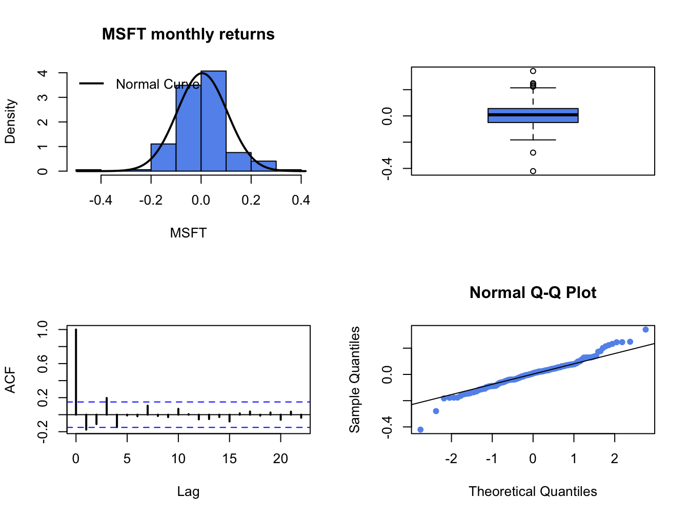
Figure 9.2: Four panel distribution plot for Microsoft monthly returns.

9.6.1.1 JB test based on skewness and kurtosis

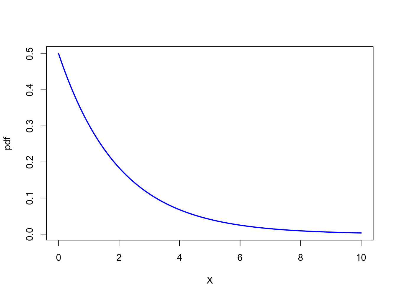
Figure 9.3: pdf of \(\chi^{2}(2)\)

In Chapter 2, we showed that the skewness and kurtosis of a normally distributed random variable are equal to zero and three, respectively. We can use this information to develop a simple test of (9.28) against (9.29) based on testing the hypotheses: \[\begin{eqnarray} H_{0}:\mathrm{skew}(R_{t}) & = & 0\,\,\,\mathrm{and}\,\,\,\mathrm{kurt}(R_{t})=3\,\,vs.\,\,\tag{9.30}\\ H_{1}:\mathrm{skew(}R_{t}) & \neq & 0\,\,\,\mathrm{or}\,\,\,\mathrm{kurt}(R_{t})\neq3\,\,\,\mathrm{or}\,\,\,\mathrm{both}.\tag{9.31} \end{eqnarray}\] To develop a test statistic for testing (9.30) against (9.31), Jarque and Bera (1981) used the result (see Kendall and Stuart, 1977) that if \(\{R_{t}\}\sim\mathrm{iid}\,N(\mu,\sigma^{2})\) then by the CLT it can be shown that: \[ \left(\begin{array}{c} \widehat{\mathrm{skew}}_{r}\\ \widehat{\mathrm{kurt}}_{r}-3 \end{array}\right)\sim N\left(\left(\begin{array}{c} 0\\ 0 \end{array}\right),\left(\begin{array}{cc} \frac{6}{T} & 0\\ 0 & \frac{24}{T} \end{array}\right)\right), \] for large enough \(T\), where \(\widehat{\mathrm{skew}}_{r}\) and \(\widehat{\mathrm{kurt}}_{r}\) denote the sample skewness and kurtosis of the returns \(\{r_{t}\}_{t=1}^{T}\), respectively. This motivates Jarque and Bera’s JB statistic: \[\begin{equation} \mathrm{JB}=T\times\left[\frac{\left(\widehat{\mathrm{ske}w}_{r}\right)^{2}}{6}+\frac{\left(\widehat{\mathrm{kurt}}_{r}-3\right)^{2}}{24}\right],\tag{9.32} \end{equation}\] to test (9.28) against (9.29). If returns are normally distributed then \(\widehat{\mathrm{skew}}_{r}\approx0\) and \(\widehat{\mathrm{kurt}}_{r}-3\approx0\) so that \(\mathrm{JB}\approx0\). In contrast, if returns are not normally distributed then \(\widehat{\mathrm{skew}}_{r}\neq0\) or \(\widehat{\mathrm{kurt}}_{r}-3\neq0\) or both so that \(\mathrm{JB}>0\). Hence, if JB is big then there is data evidence against the null hypothesis that returns are normally distributed.

To determine the critical value for testing (9.28) at a given significance level we need the distribution of the JB statistic (9.32) under the null hypothesis (9.28). To this end, Jarque and Bera show, assuming (9.28) and large enough \(T\), that: \[ \mathrm{JB}\sim\chi^{2}(2), \] where \(\chi^{2}(2)\) denotes a chi-square distribution with two degrees of freedom (see Appendix). Hence, the critical values for the JB statistic are the upper quantiles of \(\chi^{2}(2)\). Figure 9.3 shows the pdf of \(\chi^{2}(2)\). The 90%, 95% and 99% quantiles can be computed using the R function qchisq():

 qchisq(c(0.90, 0.95, 0.99), 2)

## [1] 4.61 5.99 9.21

Since the 95% quantile of \(\chi^{2}(2)\) is \(5.99\approx6\), a simple rule of thumb is to reject the null hypothesis (9.28) at the 5% significance level if the JB statistic (9.32) is greater than 6.

Let \(X\sim\chi^{2}(2)\). The p-value of the JB test is computed using: \[ p-value=\Pr(X>JB). \] If the p-value() is less than \(\alpha\) then the null () is rejected at the

Example 9.10 (Using the JB statistic to test the normality assumption for returns on Microsoft, Starbucks and the S&P 500 index)

The sample skewness and excess kurtosis values for the monthly returns on Microsoft, Starbucks, and the S&P 500 index are

skewhat = skewness(gwnMonthlyRetC) 
ekurthat = kurtosis(gwnMonthlyRetC) 
rbind(skewhat, ekurthat)

##                    MSFT   SBUX SP500
## Skewness        -0.0901 -0.987 -0.74
## Excess Kurtosis  2.0802  3.337  1.07

The sample skewness values for the assets are not too large but the sample excess kurtosis values are fairly large. The JB statistics for the three assets are easy to compute

n.obs = nrow(gwnMonthlyRetC) 
JB = n.obs*((as.numeric(skewhat)^2)/6 + (as.numeric(ekurthat)^2)/24) 
names(JB) = colnames(gwnMonthlyRetC) 
JB

##  MSFT  SBUX SP500 
##  31.2 107.7  23.9

Since all JB values are greater than 6, we reject the null hypothesis that the monthly returns are normally distributed.

You can also use the tseries function jarque.bera.test() to compute the JB statistic:

jarque.bera.test(gwnMonthlyRetC[, 1])

## 
##  Jarque Bera Test
## 
## data:  gwnMonthlyRetC[, 1]
## X-squared = 31, df = 2, p-value = 2e-07

jarque.bera.test(gwnMonthlyRetC[, 2])

## 
##  Jarque Bera Test
## 
## data:  gwnMonthlyRetC[, 2]
## X-squared = 108, df = 2, p-value <2e-16

jarque.bera.test(gwnMonthlyRetC[, 3])

## 
##  Jarque Bera Test
## 
## data:  gwnMonthlyRetC[, 3]
## X-squared = 24, df = 2, p-value = 7e-06

The test statistics are slightly different from the direct calculation above due to differences in how the sample skewness and sample kurtosis is computed within the function jarque.bera.test().

\(\blacksquare\)

9.6.1.2 Shipiro Wilks test

To be complete…

9.6.2 Tests for no autocorrelation

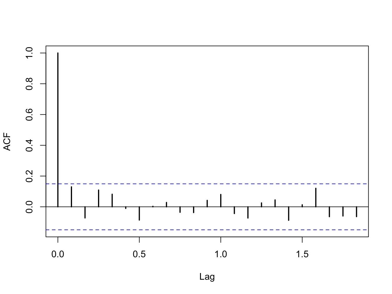
Figure 9.4: SACF for monthly returns on the S&P 500 index.

A key assumption of the GWN model is that returns are uncorrelated over time (not autocorrelated). In efficient financial markets where prices fully reflect true asset value, returns of actively traded assets should not be autocorrelated. In addition, if returns are autocorrelated then they are predictable. That is, future returns can be predicted from the past history of returns. If this is the case then trading strategies can be easily developed to exploit this predictability. But if many market participants act on these trading strategies then prices will adjust to eliminate any predictability in returns. Hence, for actively traded assets in well functioning markets we expect to see that the returns on these assets are uncorrelated over time.

For less frequently traded assets returns may appear to be autocorrelated due to stale pricing.

As we saw in Chapter 6, this allows us to aggregate the GWN model over time and, in particular, derive the square-root-of time rule for aggregating return volatility. If returns are substantially correlated over time (i.e., autocorrelated) then the square-root-of-time rule will not be an accurate way to aggregate volatility.

To measure autocorrelation in asset returns \(\{R_{t}\)} we use the j\(^{th}\) lag autocorrelation coefficient \[\begin{align*} \rho_{j} & =\mathrm{cor}(R_{t},R_{t-j})=\frac{\mathrm{cov}(R_{t},R_{t-j})}{\mathrm{var}(R_{t})}, \end{align*}\] which is estimated using the sample autocorrelation \[ \hat{\rho}_{j}=\frac{\frac{1}{T-1}\sum_{t=j+1}^{T}(r_{t}-\hat{\mu})(r_{t-j}-\hat{\mu})}{\frac{1}{T-1}\sum_{t=1}^{T}(r_{t}-\hat{\mu})^{2}}. \] In chapter 5, we used the sample autocorrelation function (SACF) to graphically evaluate the data evidence on autocorrelation for daily and monthly returns. For example, Figure 9.4 shows the SACF for the monthly returns on the S&P 500 index. Here we see that none of the \(\hat{\rho}_{j}\)values are very large. We also see a pair of blue dotted lines on the graph. As we shall see, these dotted lines are related to critical values for testing the null hypothesis that \(\rho_{j}=0\). Hence, if

9.6.2.1 Individual tests

Individual tests for autocorrelation are similar to coefficient tests discussed earlier and are based on testing the hypotheses \[ H_{0}:\rho_{j}=0\,\,\,vs.\,\,\,H_{1}:\rho_{j}\neq0, \] for a given lag \(j\). The tests rely on the result, justified by the CLT if \(T\) is large enough, that if returns are covariance stationary and uncorrelated then \[\begin{align*} \hat{\rho}_{j}\sim N\left(0,\frac{1}{T}\right)\text{ for all }j\geq1\,\mathrm{and}\,\mathrm{se}(\hat{\rho}_{j})=\frac{1}{\sqrt{T}}. \end{align*}\] This motivates the test statistics \[ t_{\rho_{j=0}}=\frac{\hat{\rho}_{j}}{\mathrm{se}(\hat{\rho}_{j})}=\frac{\hat{\rho}_{j}}{1/\sqrt{T}}=\sqrt{T}\hat{\rho}_{j},\,j\geq1 \] and the 95% confidence intervals \[ \hat{\rho}_{j}\pm2\cdot\frac{1}{\sqrt{T}}. \] If we use a 5% significance level, then we reject the null hypothesis \(H_{0}:\rho_{j}=0\) if \[ |t_{\rho_{j=0}}|=\left\vert \sqrt{T}\hat{\rho}_{j}\right\vert >2. \] That is, reject if \[ \hat{\rho}_{j}>\frac{2}{\sqrt{T}}\text{ or }\hat{\rho}_{j}<\frac{-2}{\sqrt{T}}. \] Here we note that the dotted lines on the SACF are at the points \(\pm2\cdot\frac{1}{\sqrt{T}}\). If the sample autocorrelation \(\hat{\rho}_{j}\) crosses either above or below the dotted lines then we can reject the null hypothesis \(H_{0}:\rho_{j}=0\) at the 5% level.

9.6.2.2 Joint tests

• Have to be careful how to interpret the individual tests. Cannot simply use 20 individual tests at the 5% level to test a joint hypothesis at the 5% level. With independent individual tests each test has a 5% probability of rejecting the null when it is true. So if you do 20 individual tests it would not be surprising if one tests rejects and this could be purely by chance (a type I error) if the null of no autocorrelation was true.

To be complete

9.6.3 Tests for constant parameters

A key assumption of the GWN model is that returns are generated from a covariance stationary time series process. As a result, all of the parameters of the GWN model are constant over time. However, as shown in Chapter 5 there is evidence to suggest that the assumption of covariance stationarity may not always be appropriate. For example, the volatility of returns for some assets does not appear to be constant over time.

A natural null hypothesis associated with the covariance stationarity assumption for the GWN model for an individual asset return has the form: \[ H_{0}:\mu_{i},\sigma_{i},\rho_{ij}\, \text{are constant over time}. \] To reject this null implied by covariance stationarity, one only needs to find evidence that at least one parameter is not constant over time.

9.6.3.1 Formal tests (two parameter structural change)

To be completed

• Do two-sample structural change tests based on known segments. Analysis is very similar to testing equality of parameters across two assets.

9.6.4 Tests for constant parameters based on rolling estimators

In Chapter 5 we introduced rolling descriptive statistics to informally investigate the assumption of covariance stationarity. Given any parameter \(\theta\) of the GWN model (or any function of the parameters), we can compute a set of rolling estimates of \(\theta\) over windows of length \(n<T\): \(\{\hat{\theta}_t(n) \}_{t=n}^{T}\). A time plot of these rolling estimates may show evidence of non-stationary behavior in returns.

However, one must always keep in mind that estimates have estimation error and part of the observed time variation in the rolling estimates \(\{\hat{\theta}_t(n) \}_{t=n}^{T}\) is due to random estimation error. To account for this estimation error, rolling estimates are often displayed with estimated standard error bands of the form:

\[\begin{equation} \hat{\theta}_t(n) \pm c\times \widehat{\mathrm{se}}\left( \hat{\theta}_t(n)\right), \tag{9.33} \end{equation}\]

where \(c\) is a constant representing some multiple of the estimated standard error. Typically, \(c\) is chosen so that (9.33) represents an approximate confidence interval for \(\theta\). For example, setting \(c=2\) gives an approximate 95% confidence interval.

Example 9.11 ()

As in Chapter 5, we compute 24-month rolling estimates of \(\mu\) and \(\sigma\) for Microsoft, Starbucks and the S&P 500 index using the zoo function rollapply():

roll.muhat = rollapply(gwnMonthlyRetC, width = 24, by = 1, 
                       by.column = TRUE, FUN = mean, align = "right")
roll.sigmahat = rollapply(gwnMonthlyRetC, width = 24, by = 1, 
                          by.column = TRUE, FUN = sd, align = "right")

Estimated standard errors for \(\hat{\mu}_t(n)\) and \(\hat{\sigma}_t(n)\) are computed using: \[ \widehat{\mathrm{se}}(\hat{\mu}_t(n)) = \frac{\hat{\sigma}_t(n)}{\sqrt{T}}, ~ \widehat{\mathrm{se}}(\hat{\sigma}_t(n)) = \frac{\hat{\sigma}_t(n)}{\sqrt{2T}} \] Figure 9.5 shows the rolling estimates of \(\mu\) (top panel) and \(\sigma\) (bottom panel) for Starbucks together with 95% confidence intervals (\(\pm2\times\) standard error bands) computed using:

se.muhat.SBUX = roll.sigmahat[, "SBUX"]/sqrt(24)
se.sigmahat.SBUX = roll.sigmahat[, "SBUX"]/sqrt(2 * 24)
lower.muhat.SBUX = roll.muhat[, "SBUX"] - 2 * se.muhat.SBUX
upper.muhat.SBUX = roll.muhat[, "SBUX"] + 2 * se.muhat.SBUX
lower.sigmahat.SBUX = roll.sigmahat[, "SBUX"] - 2 * se.sigmahat.SBUX
upper.sigmahat.SBUX = roll.sigmahat[, "SBUX"] + 2 * se.sigmahat.SBUX
# plot estimates with standard error bands
dataToPlot = merge(roll.muhat[, "SBUX"], lower.muhat.SBUX, 
                   upper.muhat.SBUX, roll.sigmahat[,"SBUX"],
                   lower.sigmahat.SBUX, upper.sigmahat.SBUX)
my.panel <- function(...) {
  lines(...)
  abline(h = 0)
}
plot.zoo(dataToPlot, main = "", screens = c(1, 1, 1, 2, 2, 2),
         lwd = 2, col = c("black","red", "red", "black", "red", "red"),
         lty = c("solid", "dashed", "dashed", "solid", "dashed", "dashed"),
         panel = my.panel, ylab = list("muhat", "sigmahat"))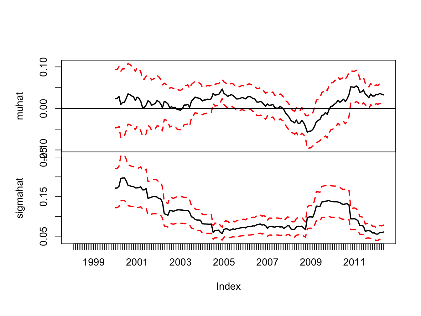

Figure 9.5: 24-month rolling estimates of \(\mu\) and \(\sigma\) for Starbucks with estimated standard error bands

The standard error bands for \(\hat{\mu}_t(n)\) are fairly wide, especially during the high volatility periods of the dot-com boom-bust and the financial crisis. During the dot-com period the 95% confidence intervals for \(\mu\) are wide and contain both positive and negative values reflecting a high degree of uncertainty about the value of \(\mu\). However, during the economic boom around 2005, where \(\hat{\mu}_t(n)\) is large and \(\hat{\sigma}_t(n)\) is small, the 95% confidence interval for \(\mu\) does not contain zero and one can infer that the mean is significantly positive. Also, at the height of the financial crisis, where \(\hat{\mu}_t(n)\) is the largest negative value, the 95% confidence interval for \(\mu\) contains all negative values and one can infer that the mean is significantly negative. At the end of the sample, the 95% confidence intervals for \(\mu\) contain all positive values.⁵²

The standard error bands for \(\hat{\sigma}_t(n)\) are smaller than the bands for \(\hat{\mu}_t(n)\) and one can see more clearly that \(\hat{\sigma}_t(n)\) significantly larger during the dot-com period and the financial crisis period than during the economic boom period and the period after the financial crisis.

\(\blacksquare\)

Plotting rolling estimates with estimated standard error bands is good practice as it reminds you that there is estimation error in the rolling estimates and part of any observed time variation is this estimation error.

9.7 Using Monte Carlo Simulation to Understand Hypothesis Testing

In chapter 7 we used Monte Carlo simulation to understand the statistical properties of estimators. Now, we will use Monte Carlo Simulation to understand hypothesis testing. To fix ideas, let \(R_{t}\) be the return on a single asset described by the GWN model, let \(\theta\) denote some parameter of the GWN model we are interested in testing an hypothesis about, let \(\hat{\theta}\) denote an estimator for \(\theta\) based on a sample of size \(T\), and let \(\widehat{\mathrm{se}}(\hat{\theta)}\) denote the estimated standard error for \(\hat{\theta}\). Suppose we are interested in testing \(H_{0}:\theta=\theta_{0}\) against \(H_{1}:\theta\neq\theta_{0}\) using the z-score \(z_{\theta=\theta_{0}}=\frac{\hat{\theta}-\theta_{0}}{\widehat{\mathrm{se}}(\hat{\theta)}}\).

To be completed

9.8 Using the Bootstrap for Hypothesis Testing

To be completed

• duality between HT and CIs can be exploited by the bootstrap. Use bootstrap to compute CI and see if hypothesized values lies in the interval. Illustrate with testing equality of 2 Sharpe ratios

9.9 Further Reading: Hypothesis Testing in the GWN Model

• Mention books by Carol Alexander for discussion of rolling and EWMA estimates
• Formal tests for structural change require advanced probability and statistics. See (Zivot 2016) for discussion. Many tests are implemented in the strucchange package.

9.10 Problems: Hypothesis Testing in the GWN Model

In this lab, you will use R to use the bootstrap to compute standard errors for GWN model estimates of five Northwest stocks in the IntroCompFin package: Amazon (amzn), Boeing (ba), Costco (cost), Nordstrom (jwn), and Starbucks (sbux). You will get started on the class project (see the Final Project under Assignments on Canvas for more details on the class project). This notebook walks you through all of the computations for the bootstrap part of the lab. You will use the following R packages

• boot
• IntroCompFinR
• PerformanceAnalytics package.
• zoo
• xts

Make sure to install these packages before you load them into R. As in the previous labs, use this notebook to answer all questions. Insert R chunks where needed. I will provide code hints below.

Reading:

• Zivot, chapters 6 (GWN Model), 7 (GWN Model Estimation) and 8 (bootstrap)
• Ruppert and Matteson, chapter 6 (resampling) and Appendix sections 10, 11, 16 and 17

Load packages and set options

suppressPackageStartupMessages(library(IntroCompFinR))
suppressPackageStartupMessages(library(corrplot))
suppressPackageStartupMessages(library(PerformanceAnalytics))
suppressPackageStartupMessages(library(xts))
options(digits = 3)
Sys.setenv(TZ="UTC")

Loading data and computing returns

Load the daily price data from IntroCompFinR, and create monthly returns over the period Jan 1998 through Dec 2014:

data(amznDailyPrices, baDailyPrices, costDailyPrices, jwnDailyPrices, sbuxDailyPrices)
fiveStocks = merge(amznDailyPrices, baDailyPrices, costDailyPrices, jwnDailyPrices, sbuxDailyPrices)
fiveStocks = to.monthly(fiveStocks, OHLC=FALSE)

## Warning in to.period(x, "months", indexAt = indexAt, name =
## name, ...): missing values removed from data

Next, let’s compute monthly continuously compounded returns using the PerformanceAnalytics function Return.Calculate()

fiveStocksRet = na.omit(Return.calculate(fiveStocks, method = "log"))
head(fiveStocksRet, n=3)

##            AMZN      BA   COST    JWN   SBUX
## Feb 1998 0.2661  0.1332 0.1193 0.1220 0.0793
## Mar 1998 0.1049 -0.0401 0.0880 0.1062 0.1343
## Apr 1998 0.0704 -0.0404 0.0458 0.0259 0.0610

We removed the missing January return using the function na.omit().

9.10.1 Exercise 9.1

Part I: GWN Model Estimation

Consider the GWN Model for cc returns

\[\begin{align} R_{it} & = \mu_i + \epsilon_{it}, t=1,\cdots,T \\ \epsilon_{it} & \sim \text{iid } N(0, \sigma_{i}^{2}) \\ \mathrm{cov}(R_{it}, R_{jt}) & = \sigma_{i,j} \\ \mathrm{cov}(R_{it}, R_{js}) & = 0 \text{ for } s \ne t \end{align}\]

where \(R_{it}\) denotes the cc return on asset \(i\) (\(i=\mathrm{AMZN}, \cdots, \mathrm{SBUX}\)).

1. Using sample descriptive statistics, give estimates for the model parameters \(\mu_i, \sigma_{i}^{2}, \sigma_i, \sigma_{i,j}, \rho_{i,j}\).

2. For each estimate of the above parameters (except \(\sigma_{i,j}\)) compute the estimated standard error. That is, compute \(\widehat{\mathrm{SE}}(\hat{\mu}_{i})\), \(\widehat{\mathrm{SE}}(\hat{\sigma}_{i}^{2})\), \(\widehat{\mathrm{SE}}(\hat{\sigma}_{i})\), and \(\widehat{\mathrm{SE}}(\hat{\rho}_{ij})\). Briefly comment on the precision of the estimates. We will compare the bootstrap SE values to these values.

9.10.2 Exercise 9.2

Part II: Bootstrapping the GWN Model Estimates

1. For each estimate of the above parameters (except \(\sigma_{i,j}\)) compute the estimated standard error using the bootstrap with 999 bootstrap replications. That is, compute \(\widehat{\mathrm{SE}}_{boot}(\hat{\mu}_{i})\), \(\widehat{\mathrm{SE}}_{boot}(\hat{\sigma}_{i}^{2})\), \(\widehat{\mathrm{SE}}_{boot}(\hat{\sigma}_{i})\), and \(\widehat{\mathrm{SE}}_{boot}(\hat{\rho}_{ij})\). Compare the bootstrap standard errors to the analytic standard errors you computed above.

2. Plot the histogram and qq-plot of the bootstrap distributions you computed from the previous question. Do the bootstrap distributions look normal?

3. For each asset, compute estimates of the \(5\%\) value-at-risk based on an initial \(\$100,000\) investment. Use the bootstrap to compute values as well as \(95\%\) confidence intervals. Briefly comment on the accuracy of the 5% VaR estimates.

9.11 Solutions to Selected Problems

In this problem, you will use R to use the bootstrap to compute standard errors for GWN model estimates of five Northwest stocks in the IntroCompFin package: Amazon (amzn), Boeing (ba), Costco (cost), Nordstrom (jwn), and Starbucks (sbux). You will get started on the class project (see the Final Project under Assignments on Canvas for more details on the class project). This notebook walks you through all of the computations for the bootstrap part of the lab. You will use the following R packages

• boot
• IntroCompFinR
• PerformanceAnalytics package.
• zoo
• xts

Make sure to install these packages before you load them into R. As in the previous labs, use this notebook to answer all questions. Insert R chunks where needed. I will provide code hints below.

Reading:

• Zivot, chapters 6 (GWN Model), 7 (GWN Model Estimation) and 8 (bootstrap)
• Ruppert and Matteson, chapter 6 (resampling) and Appendix sections 10, 11, 16 and 17

Load packages and set options

suppressPackageStartupMessages(library(IntroCompFinR))
suppressPackageStartupMessages(library(PerformanceAnalytics))
suppressPackageStartupMessages(library(xts))
suppressPackageStartupMessages(library(boot))
options(digits = 3)
Sys.setenv(TZ="UTC")

Loading data and computing returns

Load the daily price data from IntroCompFinR, and create monthly returns over the period Jan 1998 through Dec 2014:

data(amznDailyPrices, baDailyPrices, costDailyPrices, jwnDailyPrices, sbuxDailyPrices)
fiveStocks = merge(amznDailyPrices, baDailyPrices, costDailyPrices, jwnDailyPrices, sbuxDailyPrices)
fiveStocks = to.monthly(fiveStocks, OHLC=FALSE)

## Warning in to.period(x, "months", indexAt = indexAt, name =
## name, ...): missing values removed from data

Next, let’s compute monthly continuously compounded returns using the PerformanceAnalytics function Return.Calculate()

fiveStocksRet = na.omit(Return.calculate(fiveStocks, method = "log"))
head(fiveStocksRet, n=3)

##            AMZN      BA   COST    JWN   SBUX
## Feb 1998 0.2661  0.1332 0.1193 0.1220 0.0793
## Mar 1998 0.1049 -0.0401 0.0880 0.1062 0.1343
## Apr 1998 0.0704 -0.0404 0.0458 0.0259 0.0610

We removed the missing January return using the function na.omit().

Part I: GWN Model Estimation

Consider the GWN Model for cc returns

\[\begin{align} R_{it} & = \mu_i + \epsilon_{it}, t=1,\cdots,T \\ \epsilon_{it} & \sim \text{iid } N(0, \sigma_{i}^{2}) \\ \mathrm{cov}(R_{it}, R_{jt}) & = \sigma_{i,j} \\ \mathrm{cov}(R_{it}, R_{js}) & = 0 \text{ for } s \ne t \end{align}\]

where \(R_{it}\) denotes the cc return on asset \(i\) (\(i=\mathrm{AMZN}, \cdots, \mathrm{SBUX}\)).

1. Using sample descriptive statistics, give estimates for the model parameters \(\mu_i, \sigma_{i}^{2}, \sigma_i, \sigma_{i,j}, \rho_{i,j}\).

muhat.vals = apply(fiveStocksRet, 2, mean)
sigma2hat.vals = apply(fiveStocksRet, 2, var)
sigmahat.vals = apply(fiveStocksRet, 2, sd)
cov.mat = var(fiveStocksRet)
cor.mat = cor(fiveStocksRet)
covhat.vals = cov.mat[lower.tri(cov.mat)]
rhohat.vals = cor.mat[lower.tri(cor.mat)]
names(covhat.vals) <- names(rhohat.vals) <- 
  c("AMZN,BA","AMZN,COST","AMZN,JWN", "AMZN,SBUX",
    "BA,COST", "BA,JWN", "BA,SBUX",
    "COST, JWN", "COST,SBUX",
    "JWN, SBUX")

The estimates of \(\mu_i, \sigma_{i}^{2}, \sigma_i\) are

cbind(muhat.vals,sigma2hat.vals,sigmahat.vals)

##      muhat.vals sigma2hat.vals sigmahat.vals
## AMZN    0.02042        0.02814        0.1678
## BA      0.00657        0.00764        0.0874
## COST    0.01017        0.00584        0.0764
## JWN     0.01049        0.01298        0.1140
## SBUX    0.01458        0.01111        0.1054

The estimates of \(\sigma_{i,j}, \rho_{i,j}\) are

rbind(covhat.vals, rhohat.vals)

##             AMZN,BA AMZN,COST AMZN,JWN AMZN,SBUX BA,COST  BA,JWN
## covhat.vals 0.00208   0.00404  0.00714   0.00546 0.00118 0.00319
## rhohat.vals 0.14194   0.31517  0.37357   0.30862 0.17714 0.32071
##             BA,SBUX COST, JWN COST,SBUX JWN, SBUX
## covhat.vals 0.00237   0.00355   0.00271   0.00468
## rhohat.vals 0.25792   0.40724   0.33634   0.38954

2. For each estimate of the above parameters (except \(\sigma_{i,j}\)) compute the estimated standard error. That is, compute \(\widehat{\mathrm{SE}}(\hat{\mu}_{i})\), \(\widehat{\mathrm{SE}}(\hat{\sigma}_{i}^{2})\), \(\widehat{\mathrm{SE}}(\hat{\sigma}_{i})\), and \(\widehat{\mathrm{SE}}(\hat{\rho}_{ij})\). Briefly comment on the precision of the estimates. We will compare the bootstrap SE values to these values.

The SE formulas are

\[\widehat{\mathrm{SE}}(\hat{\mu}_{i})=\frac{\hat{\sigma}}{\sqrt{T}}, \widehat{\mathrm{SE}}(\hat{\sigma}_{i}^{2}) =\frac{\hat{\sigma}^2}{\sqrt{T/2}}, \widehat{\mathrm{SE}}(\hat{\sigma}_{i}) = \frac{\hat{\sigma}}{\sqrt{2T}},\widehat{\mathrm{SE}}(\hat{\rho}_{ij})=\frac{1-\hat{\rho}_{i,j}^2}{\sqrt{T}} \] The R code to compute theses estimates is

nobs = nrow(fiveStocksRet)
se.muhat = sigmahat.vals/sqrt(nobs)
se.sigma2hat = sigma2hat.vals/sqrt(nobs/2)
se.sigmahat = sigmahat.vals/sqrt(2*nobs)
se.rhohat = (1-rhohat.vals^2)/sqrt(nobs)

To interpret the SE values, it is useful to compare them to the estimates. For \(\hat{\mu}\) we have

cbind(muhat.vals, se.muhat)

##      muhat.vals se.muhat
## AMZN    0.02042  0.01177
## BA      0.00657  0.00613
## COST    0.01017  0.00536
## JWN     0.01049  0.00800
## SBUX    0.01458  0.00740

The mean values are not estimated very precisely as the SE values are almost as big as the mean estimates. BA and COST have the smallest SE values and AMZN and JWN have the largest values.

For \(\hat{\sigma}^2\) and \(\hat{\sigma}\) we have we have

cbind(sigma2hat.vals, se.sigma2hat, sigmahat.vals, se.sigmahat)

##      sigma2hat.vals se.sigma2hat sigmahat.vals se.sigmahat
## AMZN        0.02814     0.002793        0.1678     0.00833
## BA          0.00764     0.000758        0.0874     0.00434
## COST        0.00584     0.000580        0.0764     0.00379
## JWN         0.01298     0.001289        0.1140     0.00566
## SBUX        0.01111     0.001102        0.1054     0.00523

Here, we see that \(\hat{\sigma}^2\) and \(\hat{\sigma}\) are estimated more precisely as their SE values are much smaller than the estimates. Hence, we estimate volatility better than the mean.

For \(\hat{\rho}_{ij}\) we have

cbind(rhohat.vals,se.rhohat)

##           rhohat.vals se.rhohat
## AMZN,BA         0.142    0.0688
## AMZN,COST       0.315    0.0632
## AMZN,JWN        0.374    0.0604
## AMZN,SBUX       0.309    0.0635
## BA,COST         0.177    0.0680
## BA,JWN          0.321    0.0630
## BA,SBUX         0.258    0.0655
## COST, JWN       0.407    0.0585
## COST,SBUX       0.336    0.0622
## JWN, SBUX       0.390    0.0595

Here, the correlations are estimated reasonably well especially when the correlation is closer to 1.

Part II: Bootstrapping the GWN Model Estimates

1. For each estimate of the above parameters (except \(\sigma_{i,j}\)) compute the estimated standard error using the bootstrap with 999 bootstrap replications. That is, compute \(\widehat{\mathrm{SE}}_{boot}(\hat{\mu}_{i})\), \(\widehat{\mathrm{SE}}_{boot}(\hat{\sigma}_{i}^{2})\), \(\widehat{\mathrm{SE}}_{boot}(\hat{\sigma}_{i})\), and \(\widehat{\mathrm{SE}}_{boot}(\hat{\rho}_{ij})\). Compare the bootstrap standard errors to the analytic standard errors you computed above.

Here, we can use the brute force bootstrap to compute the bootstrap estimates.

B = 1000
muhat.boot = matrix(0, B, ncol(fiveStocksRet))
sigma2hat.boot = matrix(0, B, ncol(fiveStocksRet))
sigmahat.boot = matrix(0, B, ncol(fiveStocksRet))
rhohat.boot = matrix(0, B, length(rhohat.vals))
colnames(muhat.boot) = colnames(fiveStocksRet)
colnames(sigma2hat.boot) = colnames(fiveStocksRet)
colnames(sigmahat.boot) = colnames(fiveStocksRet)
colnames(rhohat.boot) = names(rhohat.vals)
n.obs = nrow(fiveStocksRet)
set.seed(123)
for (i in 1:B) {
  idx = sample(1:n.obs, replace=TRUE)
  boot.data = coredata(fiveStocksRet)[idx, ]
  muhat.boot[i, ] = apply(boot.data, 2, mean)
  sigma2hat.boot[i, ] = apply(boot.data, 2, var)
  sigmahat.boot[i, ] = apply(boot.data, 2, sd)
  cor.mat = cor(boot.data)
  rhohat.boot[i, ] = cor.mat[lower.tri(cor.mat)]
}

Then we can compute the sd values of each set of bootstrap estimates:

se.muhat.boot = apply(muhat.boot, 2, sd)
se.sigma2hat.boot = apply(sigma2hat.boot, 2, sd)
se.sigmahat.boot = apply(sigmahat.boot, 2, sd)
se.rhohat.boot = apply(rhohat.boot, 2, sd)

Compare bootsrap SE values with analytic SE values

cbind(se.muhat, se.muhat.boot)

##      se.muhat se.muhat.boot
## AMZN  0.01177       0.01200
## BA    0.00613       0.00613
## COST  0.00536       0.00554
## JWN   0.00800       0.00818
## SBUX  0.00740       0.00749

cbind(se.sigma2hat, se.sigma2hat.boot)

##      se.sigma2hat se.sigma2hat.boot
## AMZN     0.002793           0.00465
## BA       0.000758           0.00115
## COST     0.000580           0.00144
## JWN      0.001289           0.00203
## SBUX     0.001102           0.00189

cbind(se.sigmahat, se.sigmahat.boot)

##      se.sigmahat se.sigmahat.boot
## AMZN     0.00833          0.01370
## BA       0.00434          0.00658
## COST     0.00379          0.00924
## JWN      0.00566          0.00889
## SBUX     0.00523          0.00894

2. Plot the histogram and qq-plot of the bootstrap distributions you computed from the previous question. Do the bootstrap distributions look normal?

Mean: histograms

par(mfrow=c(3,2))
hist(muhat.boot[, 1], main=colnames(muhat.boot)[1], col="cornflowerblue")
hist(muhat.boot[, 2], main=colnames(muhat.boot)[2], col="cornflowerblue")
hist(muhat.boot[, 3], main=colnames(muhat.boot)[3], col="cornflowerblue")
hist(muhat.boot[, 4], main=colnames(muhat.boot)[4], col="cornflowerblue")
hist(muhat.boot[, 5], main=colnames(muhat.boot)[5], col="cornflowerblue")
par(mfrow=c(1,1))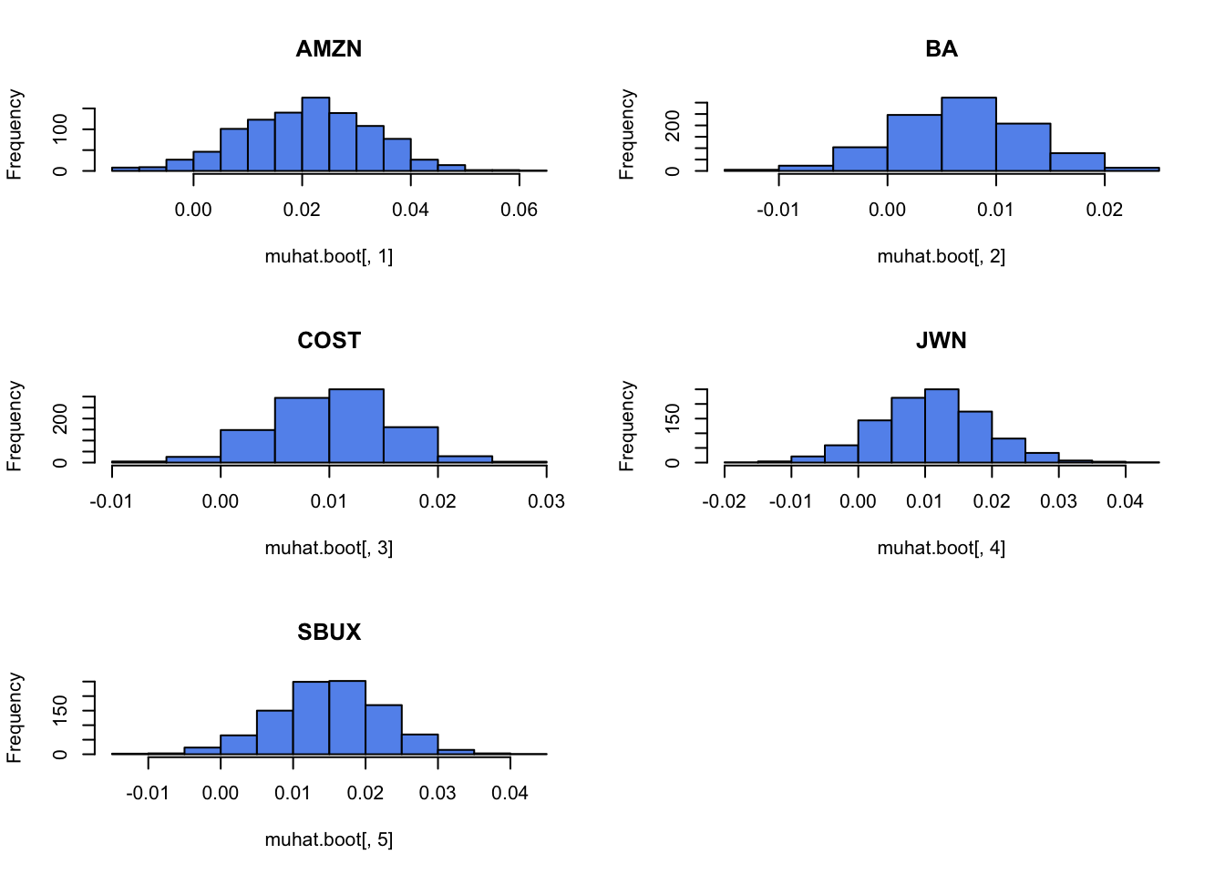

Histograms look nice and symmetric and bell-shaped.

Mean: normal QQ-plots

par(mfrow=c(3,2))
qqnorm(muhat.boot[, 1], main=colnames(muhat.boot)[1], col="cornflowerblue")
qqline(muhat.boot[, 1])
qqnorm(muhat.boot[, 2], main=colnames(muhat.boot)[2], col="cornflowerblue")
qqline(muhat.boot[, 2])
qqnorm(muhat.boot[, 3], main=colnames(muhat.boot)[3], col="cornflowerblue")
qqline(muhat.boot[, 3])
qqnorm(muhat.boot[, 4], main=colnames(muhat.boot)[4], col="cornflowerblue")
qqline(muhat.boot[, 4])
qqnorm(muhat.boot[, 5], main=colnames(muhat.boot)[5], col="cornflowerblue")
qqline(muhat.boot[, 5])
par(mfrow=c(1,1))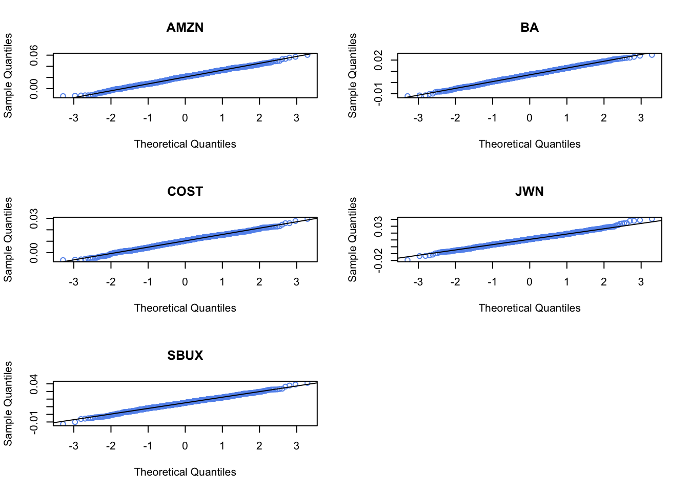

Normal QQ-plots look straight and linear.

Variance histograms

par(mfrow=c(3,2))
hist(sigma2hat.boot[, 1], main=colnames(sigma2hat.boot)[1], col="cornflowerblue")
hist(sigma2hat.boot[, 2], main=colnames(sigma2hat.boot)[2], col="cornflowerblue")
hist(sigma2hat.boot[, 3], main=colnames(sigma2hat.boot)[3], col="cornflowerblue")
hist(sigma2hat.boot[, 4], main=colnames(sigma2hat.boot)[4], col="cornflowerblue")
hist(sigma2hat.boot[, 5], main=colnames(sigma2hat.boot)[5], col="cornflowerblue")
par(mfrow=c(1,1))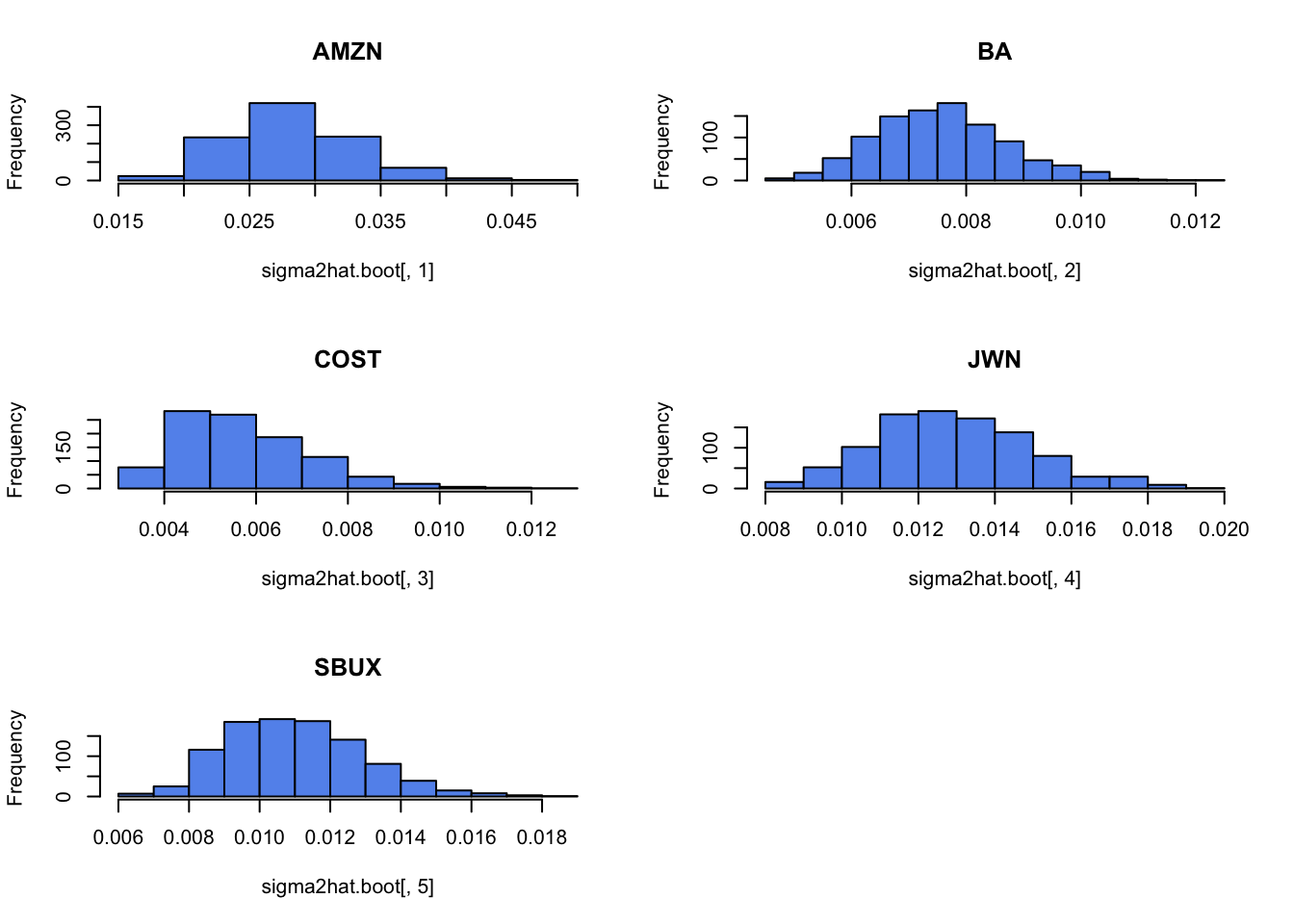

Histograms have somewhat right skewness - especially for COST, BA and SBUX (those assets with low volatility)

Variance QQ-plots

par(mfrow=c(3,2))
qqnorm(sigma2hat.boot[, 1], main=colnames(sigma2hat.boot)[1], col="cornflowerblue")
qqline(sigma2hat.boot[, 1])
qqnorm(sigma2hat.boot[, 2], main=colnames(sigma2hat.boot)[2], col="cornflowerblue")
qqline(sigma2hat.boot[, 2])
qqnorm(sigma2hat.boot[, 3], main=colnames(sigma2hat.boot)[3], col="cornflowerblue")
qqline(sigma2hat.boot[, 3])
qqnorm(sigma2hat.boot[, 4], main=colnames(sigma2hat.boot)[4], col="cornflowerblue")
qqline(sigma2hat.boot[, 4])
qqnorm(sigma2hat.boot[, 5], main=colnames(sigma2hat.boot)[5], col="cornflowerblue")
qqline(sigma2hat.boot[, 5])
par(mfrow=c(1,1))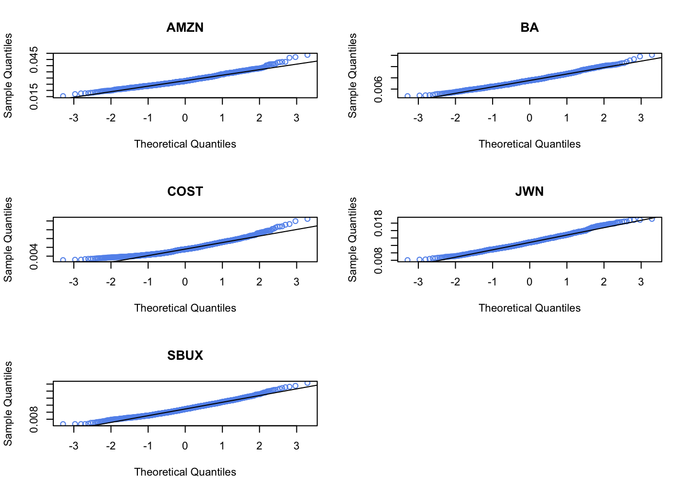

Normal QQ-plots look non-normal for BA, COST and SBUX - show right skewness.

Volatility histograms

par(mfrow=c(3,2))
hist(sigmahat.boot[, 1], main=colnames(sigmahat.boot)[1], col="cornflowerblue")
hist(sigmahat.boot[, 2], main=colnames(sigmahat.boot)[2], col="cornflowerblue")
hist(sigmahat.boot[, 3], main=colnames(sigmahat.boot)[3], col="cornflowerblue")
hist(sigmahat.boot[, 4], main=colnames(sigmahat.boot)[4], col="cornflowerblue")
hist(sigmahat.boot[, 5], main=colnames(sigmahat.boot)[5], col="cornflowerblue")
par(mfrow=c(1,1))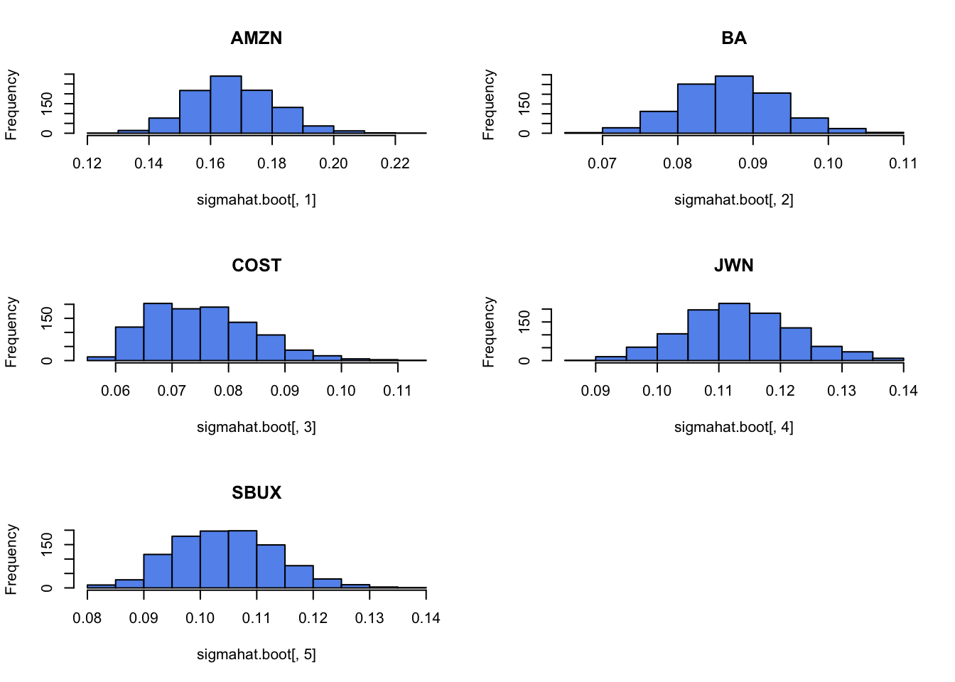

Histograms show positive skewness for BA, COST (assets with lowest volatility) and look normal for the rest.

Volatility normal QQ-plots

par(mfrow=c(3,2))
qqnorm(sigmahat.boot[, 1], main=colnames(sigmahat.boot)[1], col="cornflowerblue")
qqline(sigmahat.boot[, 1])
qqnorm(sigmahat.boot[, 2], main=colnames(sigmahat.boot)[2], col="cornflowerblue")
qqline(sigmahat.boot[, 2])
qqnorm(sigmahat.boot[, 3], main=colnames(sigmahat.boot)[3], col="cornflowerblue")
qqline(sigmahat.boot[, 3])
qqnorm(sigmahat.boot[, 4], main=colnames(sigmahat.boot)[4], col="cornflowerblue")
qqline(sigmahat.boot[, 4])
qqnorm(sigmahat.boot[, 5], main=colnames(sigmahat.boot)[5], col="cornflowerblue")
qqline(sigmahat.boot[, 5])
par(mfrow=c(1,1))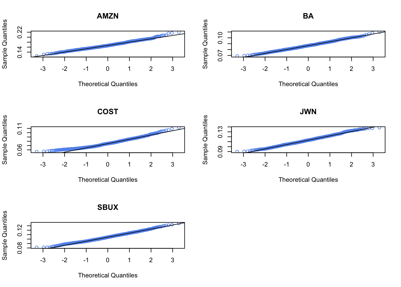

QQ-plots are not linear BA and COST and show positive skewness.

Correlation histograms

par(mfrow=c(3,2))
hist(rhohat.boot[, 1], main=colnames(rhohat.boot)[1], col="cornflowerblue", xlab="")
hist(rhohat.boot[, 2], main=colnames(rhohat.boot)[2], col="cornflowerblue")
hist(rhohat.boot[, 3], main=colnames(rhohat.boot)[3], col="cornflowerblue")
hist(rhohat.boot[, 4], main=colnames(rhohat.boot)[4], col="cornflowerblue")
hist(rhohat.boot[, 5], main=colnames(rhohat.boot)[5], col="cornflowerblue")
par(mfrow=c(1,1))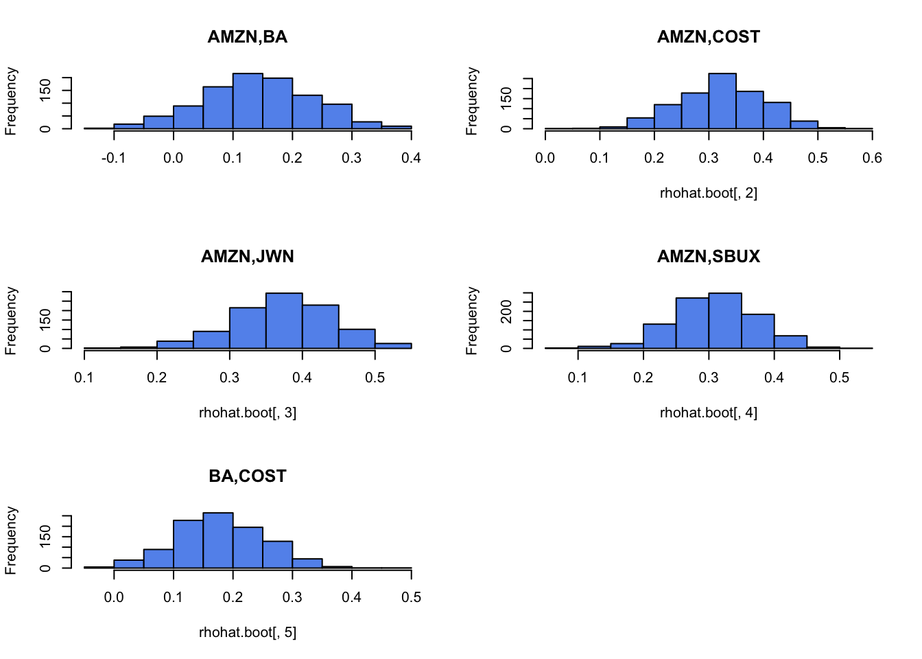

Correlation histograms look fairly symmetric.

par(mfrow=c(3,2))
hist(rhohat.boot[, 6], main=colnames(rhohat.boot)[6], col="cornflowerblue")
hist(rhohat.boot[, 7], main=colnames(rhohat.boot)[7], col="cornflowerblue")
hist(rhohat.boot[, 8], main=colnames(rhohat.boot)[8], col="cornflowerblue")
hist(rhohat.boot[, 9], main=colnames(rhohat.boot)[9], col="cornflowerblue")
hist(rhohat.boot[, 10], main=colnames(rhohat.boot)[10], col="cornflowerblue")
par(mfrow=c(1,1))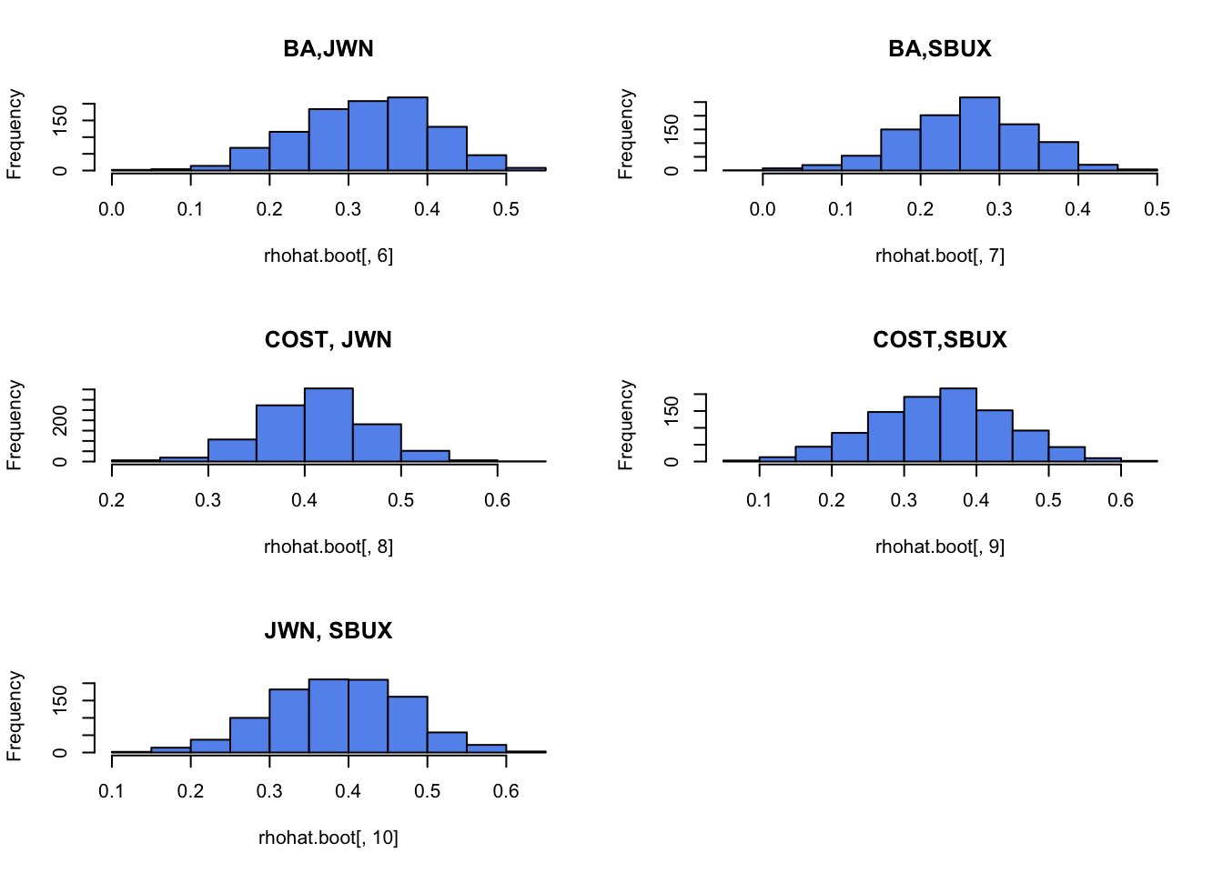

Correlation histograms look fairly symmetric.

Correlation normal QQ-plots

par(mfrow=c(3,2))
qqnorm(rhohat.boot[, 1], main=colnames(rhohat.boot)[1], col="cornflowerblue")
qqline(rhohat.boot[, 1])
qqnorm(rhohat.boot[, 2], main=colnames(rhohat.boot)[2], col="cornflowerblue")
qqline(rhohat.boot[, 2])
qqnorm(rhohat.boot[, 3], main=colnames(rhohat.boot)[3], col="cornflowerblue")
qqline(rhohat.boot[, 3])
qqnorm(rhohat.boot[, 4], main=colnames(rhohat.boot)[4], col="cornflowerblue")
qqline(rhohat.boot[, 4])
qqnorm(rhohat.boot[, 5], main=colnames(rhohat.boot)[5], col="cornflowerblue")
qqline(rhohat.boot[, 5])
par(mfrow=c(1,1))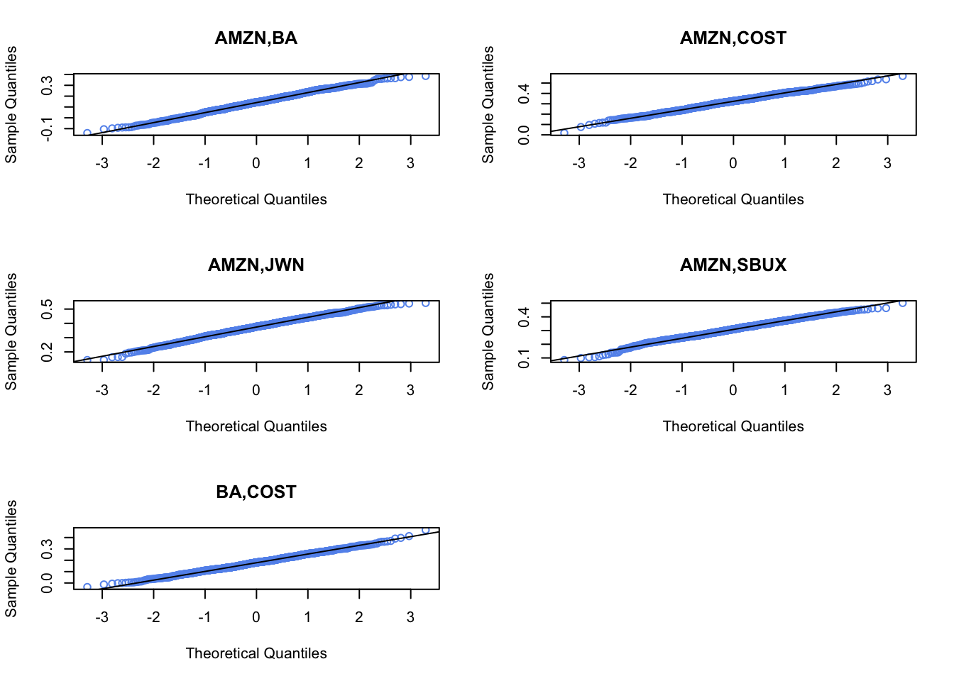

par(mfrow=c(3,2))
qqnorm(rhohat.boot[, 6], main=colnames(rhohat.boot)[6], col="cornflowerblue")
qqline(rhohat.boot[, 6])
qqnorm(rhohat.boot[, 7], main=colnames(rhohat.boot)[7], col="cornflowerblue")
qqline(rhohat.boot[, 7])
qqnorm(rhohat.boot[, 8], main=colnames(rhohat.boot)[8], col="cornflowerblue")
qqline(rhohat.boot[, 8])
qqnorm(rhohat.boot[, 9], main=colnames(rhohat.boot)[9], col="cornflowerblue")
qqline(rhohat.boot[, 9])
qqnorm(rhohat.boot[, 10], main=colnames(rhohat.boot)[10], col="cornflowerblue")
qqline(rhohat.boot[, 10])
par(mfrow=c(1,1))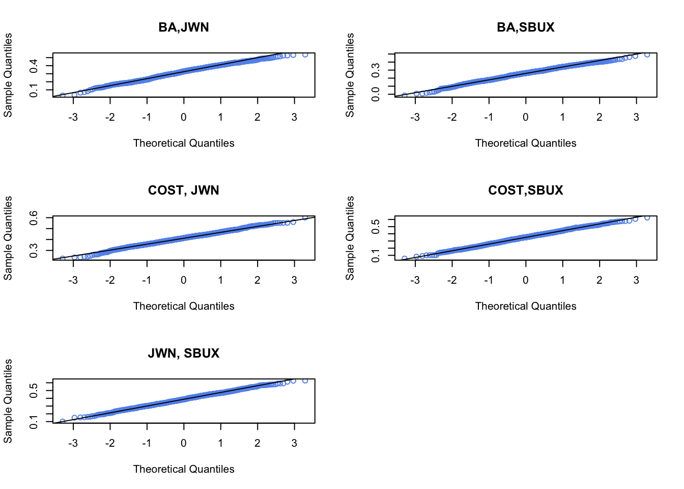

QQ-plots look pretty linear.

3. For each asset, compute estimates of the \(5\%\) value-at-risk based on an initial \(\$100,000\) investment. Use the bootstrap to compute values as well as \(95\%\) confidence intervals. Briefly comment on the accuracy of the 5% VaR estimates.

Here, we will use the boot package. First, write a function to bootstrap VaR for cc returns

# 5% Value-at-Risk
ValueAtRisk.boot = function(x, idx, p=0.05, w=100000) {
# x.mat data to be resampled
# idx       vector of scrambled indices created by boot() function
# p     probability value for VaR calculation
# w     value of initial investment
# value:
# ans       Value-at-Risk computed using resampled data

    q = mean(x[idx]) + sd(x[idx])*qnorm(p)
    VaR = (exp(q) - 1)*w
    VaR
}

Next, call the function for each asset

AMZN.VaR.boot = boot(coredata(fiveStocksRet)[, "AMZN"], statistic = ValueAtRisk.boot, R=999)
AMZN.VaR.boot

## 
## ORDINARY NONPARAMETRIC BOOTSTRAP
## 
## 
## Call:
## boot(data = coredata(fiveStocksRet)[, "AMZN"], statistic = ValueAtRisk.boot, 
##     R = 999)
## 
## 
## Bootstrap Statistics :
##     original  bias    std. error
## t1*   -22549     140        1845

Here, the boostrap SE is 1845.

Use the boot function boot.ci() to compute 95% confidence intervals:

boot.ci(AMZN.VaR.boot, conf=0.95, type=c("norm", "perc"))

## BOOTSTRAP CONFIDENCE INTERVAL CALCULATIONS
## Based on 999 bootstrap replicates
## 
## CALL : 
## boot.ci(boot.out = AMZN.VaR.boot, conf = 0.95, type = c("norm", 
##     "perc"))
## 
## Intervals : 
## Level      Normal             Percentile     
## 95%   (-26304, -19073 )   (-26093, -18929 )  
## Calculations and Intervals on Original Scale

Both intervals are very similar and show modest uncertainty in the 5% VaR values - losses from $26,00 to $19,000.

BA.VaR.boot = boot(coredata(fiveStocksRet)[, "BA"], statistic = ValueAtRisk.boot, R=999)
BA.VaR.boot

## 
## ORDINARY NONPARAMETRIC BOOTSTRAP
## 
## 
## Call:
## boot(data = coredata(fiveStocksRet)[, "BA"], statistic = ValueAtRisk.boot, 
##     R = 999)
## 
## 
## Bootstrap Statistics :
##     original  bias    std. error
## t1*   -12817    68.1        1244

Here, the boostrap SE is 1244.

Use the boot function boot.ci() to compute 95% confidence intervals:

boot.ci(BA.VaR.boot, conf=0.95, type=c("norm", "perc"))

## BOOTSTRAP CONFIDENCE INTERVAL CALCULATIONS
## Based on 999 bootstrap replicates
## 
## CALL : 
## boot.ci(boot.out = BA.VaR.boot, conf = 0.95, type = c("norm", 
##     "perc"))
## 
## Intervals : 
## Level      Normal             Percentile     
## 95%   (-15323, -10446 )   (-15247, -10302 )  
## Calculations and Intervals on Original Scale

Both intervals are very similar and show modest uncertainty in the 5% VaR values - losses from $15,00 to $10,000.

COST.VaR.boot = boot(coredata(fiveStocksRet)[, "COST"], statistic = ValueAtRisk.boot, R=999)
COST.VaR.boot

## 
## ORDINARY NONPARAMETRIC BOOTSTRAP
## 
## 
## Call:
## boot(data = coredata(fiveStocksRet)[, "COST"], statistic = ValueAtRisk.boot, 
##     R = 999)
## 
## 
## Bootstrap Statistics :
##     original  bias    std. error
## t1*   -10909     104        1660

Here, the boostrap SE is 1660.

Use the boot function boot.ci() to compute 95% confidence intervals:

boot.ci(COST.VaR.boot, conf=0.95, type=c("norm", "perc"))

## BOOTSTRAP CONFIDENCE INTERVAL CALCULATIONS
## Based on 999 bootstrap replicates
## 
## CALL : 
## boot.ci(boot.out = COST.VaR.boot, conf = 0.95, type = c("norm", 
##     "perc"))
## 
## Intervals : 
## Level      Normal             Percentile     
## 95%   (-14267,  -7760 )   (-14503,  -8094 )  
## Calculations and Intervals on Original Scale

Both intervals are very similar and show modest uncertainty in the 5% VaR values - losses from $14,00 to $7,000.

JWN.VaR.boot = boot(coredata(fiveStocksRet)[, "JWN"], statistic = ValueAtRisk.boot, R=999)
JWN.VaR.boot

## 
## ORDINARY NONPARAMETRIC BOOTSTRAP
## 
## 
## Call:
## boot(data = coredata(fiveStocksRet)[, "JWN"], statistic = ValueAtRisk.boot, 
##     R = 999)
## 
## 
## Bootstrap Statistics :
##     original  bias    std. error
## t1*   -16217    86.2        1581

Here, the boostrap SE is 1581.

Use the boot function boot.ci() to compute 95% confidence intervals:

boot.ci(JWN.VaR.boot, conf=0.95, type=c("norm", "perc"))

## BOOTSTRAP CONFIDENCE INTERVAL CALCULATIONS
## Based on 999 bootstrap replicates
## 
## CALL : 
## boot.ci(boot.out = JWN.VaR.boot, conf = 0.95, type = c("norm", 
##     "perc"))
## 
## Intervals : 
## Level      Normal             Percentile     
## 95%   (-19402, -13204 )   (-19238, -13113 )  
## Calculations and Intervals on Original Scale

Both intervals are very similar and show modest uncertainty in the 5% VaR values - losses from $19,00 to $13,000.

SBUX.VaR.boot = boot(coredata(fiveStocksRet)[, "SBUX"], statistic = ValueAtRisk.boot, R=999)
SBUX.VaR.boot

## 
## ORDINARY NONPARAMETRIC BOOTSTRAP
## 
## 
## Call:
## boot(data = coredata(fiveStocksRet)[, "SBUX"], statistic = ValueAtRisk.boot, 
##     R = 999)
## 
## 
## Bootstrap Statistics :
##     original  bias    std. error
## t1*   -14680     153        1600

Here, the boostrap SE is 1600.

Use the boot function boot.ci() to compute 95% confidence intervals:

boot.ci(SBUX.VaR.boot, conf=0.95, type=c("norm", "perc"))

## BOOTSTRAP CONFIDENCE INTERVAL CALCULATIONS
## Based on 999 bootstrap replicates
## 
## CALL : 
## boot.ci(boot.out = SBUX.VaR.boot, conf = 0.95, type = c("norm", 
##     "perc"))
## 
## Intervals : 
## Level      Normal             Percentile     
## 95%   (-17969, -11698 )   (-17807, -11670 )  
## Calculations and Intervals on Original Scale

Both intervals are very similar and show modest uncertainty in the 5% VaR values - losses from $18,00 to $12,000.

References

Zivot, E. 2016. Modeling Financial Time Series with R. New York: Springer.

---

46. In this book, we do not consider evaluating hypotheses from a Bayesian perspective.↩︎

47. As an extreme example, consider testing \(H_{0}:\textrm{"all swans are white"}\). To logically accept this hypothesis you would have to show that every swan that ever existed is white. In contrast, if you have a data set that only contains white swans then saying you cannot reject the null hypothesis that all swans are white is consistent with your data set. ↩︎

48. It is important to emphasize that there is a “true state of the world” in this context. That is, the null hypothesis \(H_{0}\) is either true or it is not. As a result, \(\Pr\left\{H_{0}\,\textrm{is true}\right\} =1\) or \(0\) depending on whether \(H_{0}\) is true or not. ↩︎

49. A capital murder trial is one in which the defendant is eligible for the death penalty.↩︎

50. Tests for model assumptions are sometimes called model specification tests.↩︎

51. This means that in an infinite number of hypothetical samples from the GWN model in which \(H_{0}\) is true only 5 percent of the samples produce an estimate \(\hat{\mu}_{i}\) that is more than \(1.96\) values of \(\mathrm{se}(\hat{\mu}_{i})\) away from \(\mu_{i}^{0}\).↩︎

52. We have to be a little careful about interpreting the implicit hypotheses tests underlying the rolling 95% confidence intervals. Each confidence interval represents a single hypothesis test with a 5% significane level. However, we have many confidence intervals and so we are really doing many hypothesis tests. The joint significance level for all of these tests will be larger than the significance level for a single test.↩︎