Chapter 8 Tests of Statistical Hypotheses
8.3 Tests About Proportions
This is section 8.3 in your book.
The traditional procedure (which gives a Wald statistic) is based on a \(z\) test statistic that has a standard normal distribution \(Z \sim N(0,1)\) under the null and \(p\)-values are computed using the standard normal distribution. This is available on the TI calculators as 1PropZTest and in R as prop.test. The R function reports the test statistic as \(X^2\) which has a chi-square distribution with \(df=1\). Note that squaring a standard normal distribution results in a chi-square distribution with \(df=1\)
\[z=\frac{\hat{p}-p_O}{\sqrt{\frac{p_O(1-p_O)}{n}}}\] Six Step Method for Hypothesis Testing
I will be presenting hypothesis testing via a systematic six step process (your book presents it as a four step process that basically combines my first three steps into one), and will expect you to use these steps when you work problems. I will work through our first example slowly and in great detail, since there is a lot of new concepts and terminology to discuss.
Step One: Write Hypotheses
For our first example, suppose that we have a coin that we suspect is unfair (i.e. the coin will not give us heads 50% of the time if we flip it many times). This research question will be turned into a pair of mathematical statements called the null and alternative hypotheses. Hypotheses are statements about the value of a parameter, not a statistic.
The null hypothesis, or \(H_O\), states that there is no difference (or effect) from the population parameter (hypothesized value) and is what will be statistically tested. The alternative hypothesis, or \(H_A\), states that there is some sort of difference (or effect) from that parameter. The alternative will typically correspond to one’s research hypothesis.
\[H_O: p=0.50\] \[H_A: p \neq 0.50\]
For our artificial first example, the null hypothesis is stating that our coin is fair (gives heads 50% of the time), while the alternative hypothesis is stating that the coin is unfair and does not give heads 50% of the time. This is an example of a two-sided hypothesis, also called a non-directional hypothesis. It is two-sided (non-directional) because we have NOT indicated any sort of a priori belief that the coin was biased to give either more than 50% or fewer than 50% heads when flipped.
In many research situations, we will have a one-sided or directional hypothesis. For example, a medical study might look to see if a treatment will significantly lower the average blood pressure of patients when compared to a control. I will illustrate both possible directions, first if we think the coin is biased in favor of heads.
\[H_O: p=0.50\]
\[H_A: p>0.50\]
Next, consider if we thought the coin was biased in favor of tails.
\[H_O: p=0.50\]
\[H_A: p<0.50\]
Step Two: Choose Level of Significance
This is where you choose your value for \(\alpha\) (usually 0.05), thereby setting the risk one is willing to take of rejecting the null hypothesis when it is actually true (i.e. declaring that you found a significant effect that in fact does not exist).
\[\alpha=0.05\]
A two-sided hypothesis test at level \(\alpha\) will correspond to a \(100(1-\alpha)\%\) confidence interval.
Step Three: Choose Your Test and Check Assumptions This is where you choose your ‘tool’ (i.e. test) and check the mathematical assumptions of that test to make sure you are using the proper ‘tool’ for the job. For the one-proportion \(z\)-test, the assumptions are:
- the data is from a random sample
- the data values are independent
- the sample size is sufficient to use the normal approximation to the binomial
Checking the first two conditions involves judging whether or not the sampling was done in a random and independent fashion. The third condition can be judged mathematically.
Suppose we plan on flipping the coin \(n=400\) times. These flips will clearly be random and independent. We can check to make sure that both the expected number of successes AND the expected number of failures are at least 10; check that \(np_O \geq 10\) and \(nq_0 \geq 10\). In our example, \(n=400\), \(p_O=0.5\) and \(q_O=1-p_O=1-0.5=0.5\), so we have 200 expected successes and 200 expected failures, more than enough, and we may proceed.
Step Four: Calculate the Test Statistic This is what you thought stats class was all about. You will use a formula (or an appropriate function on a calculator or software package) to compute a test statistic based on observed data. The test statistic for this test is:
\[z = \frac{\hat{p}-p_O}{\sqrt{\frac{p_O q_O}{n}}}\]
Suppose we obtain \(X=215\) heads in \(n=400\) flips, such that \(\hat{p}=\frac{215}{400}=0.5375\). Our test statistic will be:
\[z = \frac{.5375-.5}{\sqrt{\frac{0.5(0.5)}{400}}}=\frac{0.0375}{0.025}=1.5\]
The distribution of this test statistic \(z\) will be \(z \sim N(0,1)\) (i.e. standard normal) WHEN the null hypothesis is true.
Step Five: Make a Statistical Decision This is where you either determine the decision rule (‘old-school’) or compute a \(p\)-value (‘new-school’) and decide whether to reject or fail to reject the null hypothesis.
Step Five: Make a Statistical Decision (via the Decision Rule)
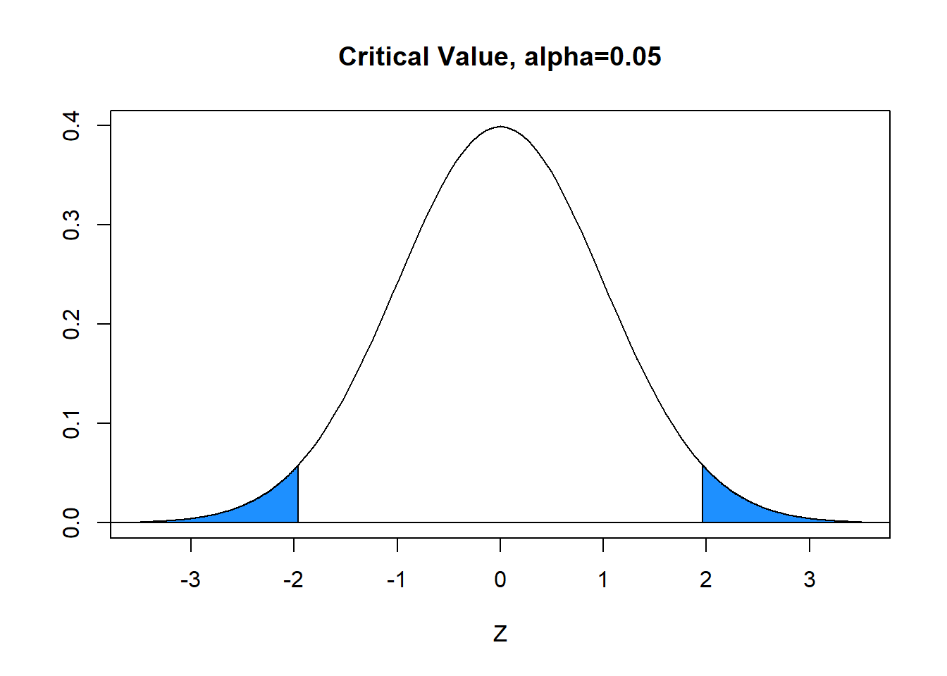
With \(\alpha=0.05\) (area in blue), the critical value is \(z^*=1.96\). The blue tails in the graph below each have area=\(\alpha/2=.025\) and the white area between is equal to \(1-\alpha=0.95\). Hence, the decision rule is to reject \(H_0\) when the absolute value of the computed test statistic \(z\) exceeds critical value \(z^*\), or reject \(H_0\) if \(|z|>z^*\). In our problem, \(|z|=1.50 \not > 1.96=z^*\) and we FAIL TO REJECT the null.
Step Five: Make a Statistical Decision (via the \(p\)-value)
When you use technology, a statistic called the p-value will be computed, based on your computed test statistic. The \(p\)-value is defined to be the probability of obtaining a value as extreme as our test statistic, IF the null hypothesis is true. For our two-sided \(z\)-test,
\[ \begin{aligned} \text{p-value}= & P(|z|>1.50) \\ = & 2 \times P(z<-1.50) \\ = & 2 \times P(z>1.50) \\ = & 2 \times 0.0668 \\ = & 0.1336 \end{aligned} \] (area in red)
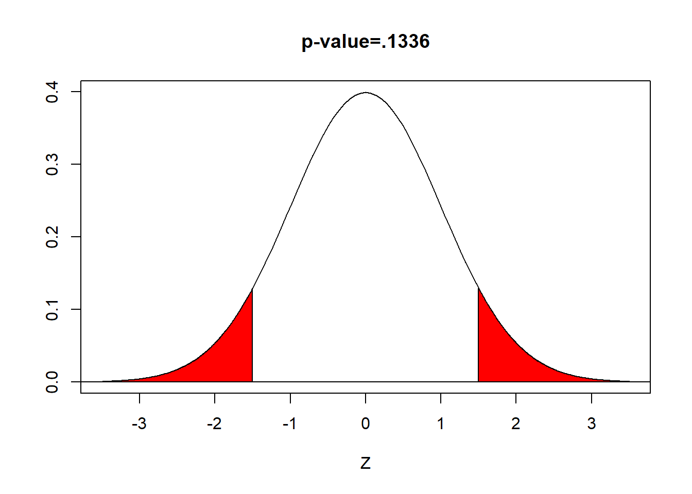
When the \(p\)-value is less than \(\alpha\), we reject the null hypothesis. We have ‘evidence beyond a reasonable doubt’.
When the \(p\)-value is greater than or equal to \(\alpha\), we fail to reject the null. We do not have ‘evidence beyond a reasonable doubt’.
Here \(.1336>.05\) and we fail to reject the null hypothesis
Step Six: Conclusion This is where you explain what all of this means to your audience. The terminology you use should be appropriate for the audience.
Since we rejected the null hypothesis, a proper conclusion would be:
The proportion of coin flips that are heads is NOT significantly different than 0.50. In other words, we do not have evidence to show the coin is unfair.
Remember, the amount of statistical jargon that you use in your conclusion depends on your audience! If your audience is a committee of professors, you can use more terminology than if your audience is someone like a school principal or hospital administrator or the general public.
Here’s the code for this test in R, using the function prop.test. The function 1-PropZTest on the TI-84 calculator does the same.
x <- 215  # number of successes
n <- 400  # sample size
p.hat <- x/n # sample statistic
p.null <- 0.5 # null hypothesis

z <- (p.hat-p.null)/sqrt(p.null*(1-p.null)/n)
z # test statistic
## [1] 1.5## [1] 2.25## [1] 0.1336144## [1] 0.1336144# built in R function, uses chi-squared rather than z
# the 1-PropZTest function on the TI-84 calculator uses the z statistic
prop.test(x=x,n=n,alternative="two.sided",correct=FALSE)##
## 1-sample proportions test without continuity correction
##
## data: x out of n
## X-squared = 2.25, df = 1, p-value = 0.1336
## alternative hypothesis: true p is not equal to 0.5
## 95 percent confidence interval:
## 0.4885138 0.5857727
## sample estimates:
## p
## 0.53758.4 Tests About One Mean
This is section 8.1 in your book.
A \(z\)-test similar to the \(z\)-interval for a mean exists, but depends on the strong assumptions that the data is normally distributed AND we know the true value of the \(\sigma\) parameter. In most situations, we would not know the true value for \(\sigma\). The sample standard deviation \(s\) still seems like a natural choice to use in place of \(\sigma\) in our confidence interval formulas.
We will compute a test statistic \[t=\frac{\bar{x}-\mu_0}{s/\sqrt{n}}\]
This statistic will follow a \(t\)-distribution with \(df=n=1\) when the null is true, and we will determine the \(p\)-value based on that \(t\)-distribution.
Suppose we have a sample of \(n=16\) seven-year-old boys from Kentucky. We have a hypothesis that these boys will be heavier than the national average of \(\mu=52\) pounds. We will not assume that we have `magical’ knowledge about the value of \(\sigma\) or whether this data is normally distributed or not.
Since we are not assuming that the variance is known, the \(z\)-test is no longer the proper `tool’; we will reach into our toolbox and use the one-sample \(t\)-test instead.
##  min Q1 median Q3 max    mean       sd  n missing
##   45 48     54 59  95 56.4375 11.87697 16       0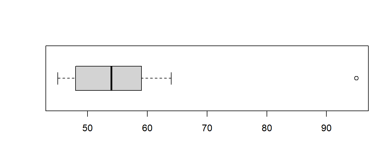
One boy seems to be an outlier. Maybe he is obese or just very tall for his age. This data point might cause the distribution to be skewed and affect our ability to use the \(t\)-test!
I am using the boxplot as an informal check of the ‘normality’ of the data. In reality, I’m just hoping that the data is reasonably symmetric and is not skewed, but the outlier is making this assumption untenable.
What to do about outliers?
Most statisticians do not consider it appropriate to delete an outlier unless there is both a statistical and a non-statistical reason for that deletion. Outliers can occur for several reasons: there might have been a data entry error (maybe that 95 was really 59), that observation might not belong to the population (maybe that boy was actually 13 years old), or it might be a true observation (that boy is obese and/or very tall for his age).
For our example, it was a data entry error. The boy was actually 59 pounds.
##  min Q1 median   Q3 max    mean       sd  n missing
##   45 48     54 58.5  64 54.1875 6.079679 16       0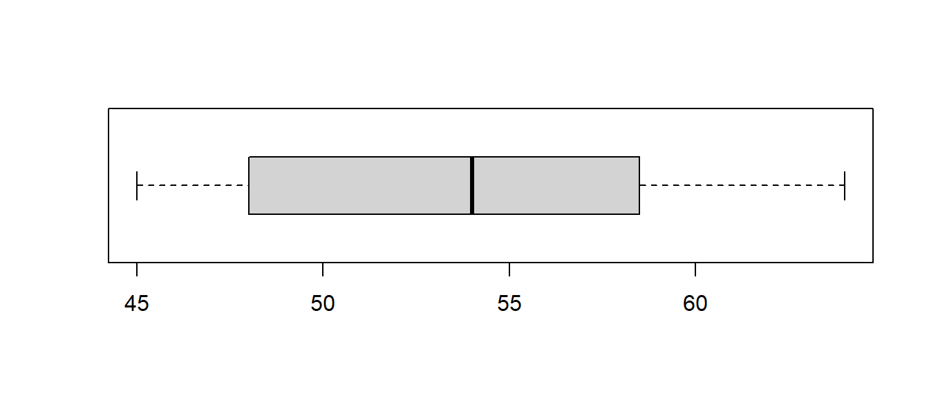
# Suppose Ho: mu=52 versus Ho: mu > 52
t.stat <- (mean(weight)-52)/(sd(weight)/sqrt(length(weight)))
t.stat
## [1] 1.439221Computation of the \(p\)-value will be more difficult for us with the \(t\)-test than the \(z\)-test. The reason is that the \(t\)-table that is generally provided in statistical textbooks is much less extensive than the standard normal table. For us to be able to compute the exact \(p\)-value for a \(t\)-test, we need to:
- Have a two page \(t\)-table similar to the normal table for every possible value of \(df\); that is, every row of the \(t\)-table would become two pages of probabilities. We do not typically have access to such tables. We can approximate the \(p\)-value with our one-page \(t\)-table.
We refer to the row for \(df=15\). Notice our test statistic \(t=1.439\) follows between the critical values \(t^*=1.341\) and \(t^*=1.753\).
Hence, our \(p\)-value is \(.05< \text{p-value} < .10\). If we had \(H_a: \mu \neq 52\), then it would be \(.10 < \text{p-value} < .20\).
- Evaluate the integral \(P(t>1.439)=\int_{1.439}^{\infty} f(x) dx\), where \(f(x)\) is the probability density function for the \(t\)-distribution with \(n-1\) df. The pdf for the \(t\)-distribution with \(r\) df is:
\[f(x)=\frac{\Gamma[(r+1)/2]}{\sqrt{\pi r}\Gamma(r/2)} \frac{1}{(1+x^2/r)^{(r+1)/2}}\] so we won’t be directly integrating this function!
- Use techonology to get the \(p\)-value; that is, let the calculator or computer do the difficult math needed to compute the \(p\)-value. With the TI-calcuator, use
tcdf(1.439,1E99,15)to get \(p=0.0853\). With R,
## [1] 0.08534527You can do this test on a TI calcuator with the 2:T-Test function under the TESTS menu after pushing the STAT key. With R:
##
##  One Sample t-test
##
## data:  weight
## t = 1.4392, df = 15, p-value = 0.08531
## alternative hypothesis: true mean is greater than 52
## 95 percent confidence interval:
##  51.523    Inf
## sample estimates:
## mean of x
##   54.1875
If you wanted a two-sided hypothesis and/or the two-sided \(100(1-\alpha)\)% confidence interval, use:
##
##  One Sample t-test
##
## data:  weight
## t = 1.4392, df = 15, p-value = 0.1706
## alternative hypothesis: true mean is not equal to 52
## 95 percent confidence interval:
##  50.94787 57.42713
## sample estimates:
## mean of x
## 54.1875##
## One Sample t-test
##
## data: weight
## t = 1.4392, df = 15, p-value = 0.1706
## alternative hypothesis: true mean is not equal to 52
## 99 percent confidence interval:
## 49.70873 58.66627
## sample estimates:
## mean of x
## 54.1875## mean of x lower upper level
## 1 54.1875 49.70873 58.66627 0.99Written up in the six-step method, we have:
Step One: Write Hypotheses
\[H_0: \mu=52\] \[H_a: \mu > 52\]
Step Two: Choose Level of Significance
Let \(\alpha=0.05\).
Step Three: Choose Test & Check Assumptions
We choose the \(t\)-test for a mean, based on having an independet random sample. After finding the data entry error, the data was reasonably symmteric and “nearly normal”, without outliers.
Step Four: Calculate the Test Statistic
\[t=\frac{\bar{x}-\mu_0}{s/\sqrt{n}}\]
\[t=\frac{54.1875-52}{6.079679/\sqrt{16}}=1.439\]
\[df=n-1=16-1=15\]
Step Five: Make a Statistical Decision
We found \(p\)-value=0.0835. This was larger than \(\alpha=0.05\), so we failed to reject the null hypothesis.
Step Six: Conclusion
Since we failed to reject the null hypothesis, a proper conclusion would be:
The mean weight of seven-year-old boys in Kentucky is NOT significantly greater than the national average of 52 pounds.
8.5 Tests of the Equality of Two Means
This is section 8.2 in your book.
Hypothesis Test for the Difference in Two Independent Means \(\mu_1-\mu_2\)
Often we want to test the difference of means between two independent groups.
For example, we want to compare the mean age of subjects assigned to the treatment group (call it \(\mu_1\)) and the mean age of subjects assigned to the control group (call it \(\mu_2\)). If we assume equal variances between the groups, the test statistic is:
\[t=\frac{\bar{x_1}-\bar{x_2}}{\sqrt{s_p^2(\frac{1}{n_1}+\frac{1}{n_2})}}\]
where \(s_p^2\), the is:
\[s_p^2=\frac{(n_1-1)s_1^2+(n_2-1)s_2^2}{n_1+n_2-2}\]
and the degrees of freedom are \[df=n_1+n_2-2\]
We have a sample of \(n_1=16\) 10-year-old boys and \(n_2=14\) 10-year-old girls. The summary statistics are:
\(\bar{x_1}=55.7\) inches, \(s_1=3.2\), \(\bar{x_2}=53.2\), \(s_2=2.8\)
We are testing for a significant difference (i.e. no direction). If we had sixteen-year-olds, we would probably use a one-sided alternative stating that boys are taller than girls.
Step One: Write Hypotheses
\[H_0: \mu_1=\mu_2\] \[H_a: \mu_1 \neq \mu_2\]
Step Two: Choose Level of Significance Let \(\alpha=0.05\).
Step Three: Choose Test/Check Assumptions
I will choose the two-sample \(t\)-test. Assumptions include that the samples are independent, random, and normally distributed with equal variances. For this example, we will assume these are met without any further checks, but in practice you should check the boxplots or \(qq\)-plots to assess this.
Step Four: Compute the Test Statistic
\[s_p^2=\frac{(16-1)(3.2^2)+(14-1)(2.8^2)}{16+14-2}=\frac{255.52}{28}=9.1257\]
\[t=\frac{\bar{x_1}-\bar{x_2}}{\sqrt{s_p^2(\frac{1}{n_1}+\frac{1}{n_2})}}=\frac{55.7-53.2}{\sqrt{9.1257(\frac{1}{16}+\frac{1}{14})}}=\frac{2.5}{\sqrt{1.2222}}\]
\[t=2.261\]
\[df=n_1+n_2-2=16+14-2=28\]
Step Five: Compute the \(p\)-value
Below shows a \(t\)-table with the pertinent values highlighted. We refer to the row for \(df=28\). Notice our test statistic \(t=2.261\) follows between the critical values \(t^*=2.048\) and \(t^*=2.467\). Because we have a two-sided test, read the probability from the top of the table.
Hence, our \(p\)-value is between 0.02 and 0.05, or \(.02 < \text{p-value} < .05\).
With the TI-calcuator, use 2*tcdf(2.261,1E99,28) to get \(p=0.0317\). Or with R,
## [1] 0.03172045Since \(p < \alpha\) we reject the null hypothesis at \(\alpha=.05\). We would have failed to reject \(H_0\) if we had used \(\alpha=0.01\).
Step Six: Conclusion
There is sufficient evidence that the mean heights of 10-year old boys and girls are significantly different.
You can do this test on a TI calcuator with the 4:2-SampTTest function with Pooled:Yes under the TESTS menu after pushing the STAT key. We’ll do a different example with R shortly.
Equal Variances and Unequal Variances
The assumption of equal variances is often not met, and an alternative version of the \(t\)-test exists when we assume unequal variances. This test is often called Welch’s \(t'\)-test. On a TI calculator, changing from Pooled=Yes to Pooled=No will use Welch’s formula.
\[t'=\frac{\bar{x_1}-\bar{x_2}}{\sqrt{\frac{s^2_1}{n_1}+\frac{s^2_2}{n_2}}}\]
Notice we do not need to compute \(s_p^2\), pooled variance. However, the degrees of freedom \(\nu\) are no longer equal to \(n_1+n_2-2\). Instead, \(\nu\) is computed by an ugly formula.
\[\nu=\frac{(s_1^2/n_1+s_2^2/n_2)^2}{(s_1^2/n_1)^2/(n_1-1) + (s_2^2/n_2)^2/(n_2-1)}\]
We will use R in order to compute Welch’s \(t\)-test (unequal variances), as well as the standard two sample \(t\)-test (equal variances).
I will quickly mention that formulas for a CI for \(\mu_1-\mu_2\) exist, based on the rather unrealistic assumption that the variances of the two samples \(\sigma^1_1\) and \(\sigma^2_2\) are known (the 2-SampZInterval on the TI) and when the variances are not known.
The data set survey in the MASS package has the responses of \(n=237\) statistics students at an Australian university. We are going to determine if there is a significant difference between male and female students in terms of their pulse rate (heart beats per minute).
First, let’s look at the data:
##      Sex Wr.Hnd NW.Hnd W.Hnd    Fold Pulse    Clap Exer Smoke Height      M.I
## 1 Female   18.5   18.0 Right  R on L    92    Left Some Never 173.00   Metric
## 2   Male   19.5   20.5  Left  R on L   104    Left None Regul 177.80 Imperial
## 3   Male   18.0   13.3 Right  L on R    87 Neither None Occas     NA     <NA>
## 4   Male   18.8   18.9 Right  R on L    NA Neither None Never 160.00   Metric
## 5   Male   20.0   20.0 Right Neither    35   Right Some Never 165.00   Metric
## 6 Female   18.0   17.7 Right  L on R    64   Right Some Never 172.72 Imperial
##      Age
## 1 18.250
## 2 17.583
## 3 16.917
## 4 20.333
## 5 23.667
## 6 21.000## Sex min Q1 median Q3 max mean sd n missing
## 1 Female 40 68 75 83 104 75.12632 11.40664 95 23
## 2 Male 35 65 72 80 104 73.19792 11.99967 96 22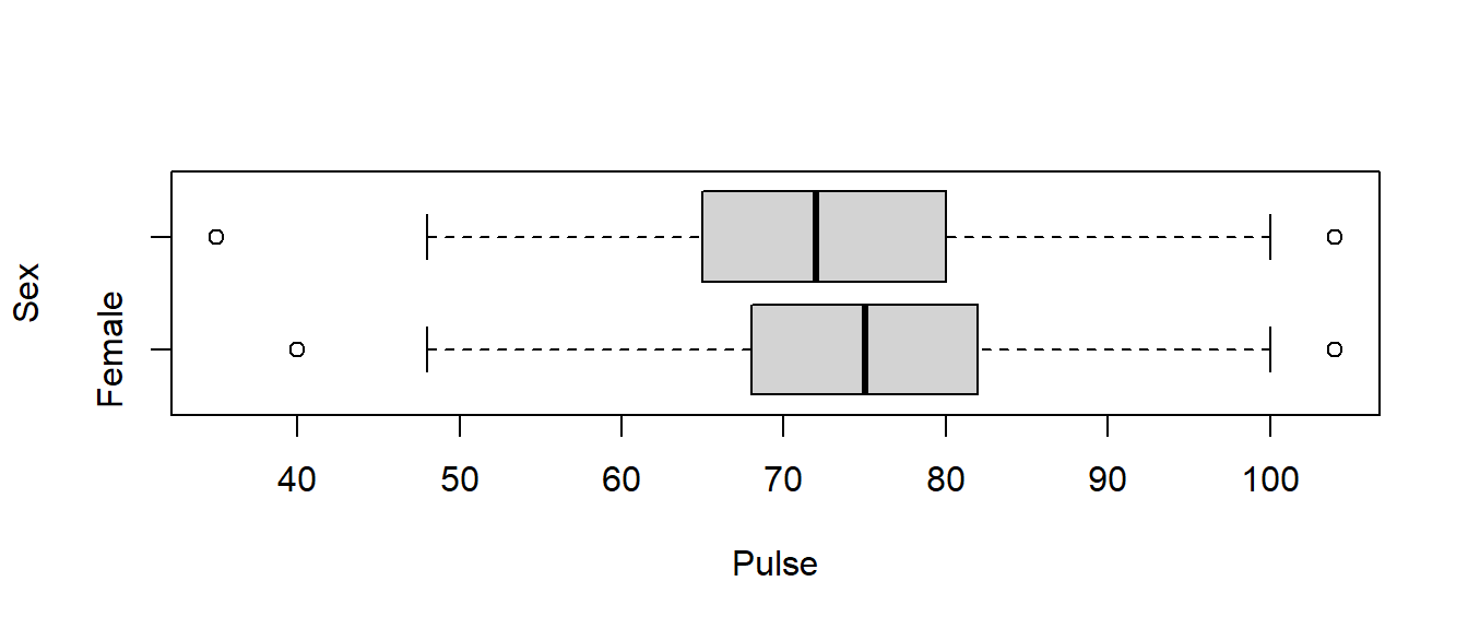
There are a few outliers in the data set, but we have large sample sizes (over 90 in each group), so I will proceed with the \(t\)-test. Even though the sample standard deviations are close to equal and using the equal variances version of the \(t\)-test would be OK, the general advice when using technology is to assume unequal variances. The two version of the \(t\)-test will be virtually identical if the variances are close to equal, but Welch’s \(t\)-test will be more accurate when the variances are unequal.
I won’t write it out in the six-step method, but my hypotheses are \(H_o: \mu_1 = \mu_2\) versus \(H_a: \mu_1 \neq \mu_2\) and I will use \(\alpha=0.10\) rather than \(\alpha=0.05\) this time.
##
##  Welch Two Sample t-test
##
## data:  Pulse by Sex
## t = 1.1384, df = 188.7, p-value = 0.2564
## alternative hypothesis: true difference in means between group Female and group Male is not equal to 0
## 90 percent confidence interval:
##  -0.8716696  4.7284678
## sample estimates:
## mean in group Female   mean in group Male
##             75.12632             73.19792
From the output, our test statistic is \(t=1.138\) with \(df \approx 188\) and the \(p\)-value of 0.2564 leads us to fail to reject the null hypothesis and conclude that there is no evidence for a difference in pulse rate between the male and female students. The 90% CI of \((-0.8717,4.7285)\) contains the null value of zero (i.e. no difference).
For comparison, I will add the option var.equal=TRUE to run the equal/pooled version of the \(t\)-test.
##
##  Two Sample t-test
##
## data:  Pulse by Sex
## t = 1.1381, df = 189, p-value = 0.2565
## alternative hypothesis: true difference in means between group Female and group Male is not equal to 0
## 90 percent confidence interval:
##  -0.8723938  4.7291920
## sample estimates:
## mean in group Female   mean in group Male
##             75.12632             73.19792
You can see the results are virtually identical.
Suppose we looked at the student’s height (in cm), instead. We would probably expect a significant difference between the sexes (and the large \(t\) test statistic and tiny \(p\)-value substantiates this belief), and a somewhat larger difference in variances. In fact the sample variance of men is nearly twice that of women.
\[s^2_F=6.151777^2=37.84, s^2_M=8.380252^2=70.23\]
I’ll compute both versions of the \(t\)-test with corresponding 95% confidence intervals.
##      Sex    min     Q1 median  Q3    max     mean       sd   n missing
## 1 Female 150.00 162.56 166.75 170 180.34 165.6867 6.151777 102      16
## 2   Male 154.94 172.72 180.00 185 200.00 178.8260 8.380252 106      12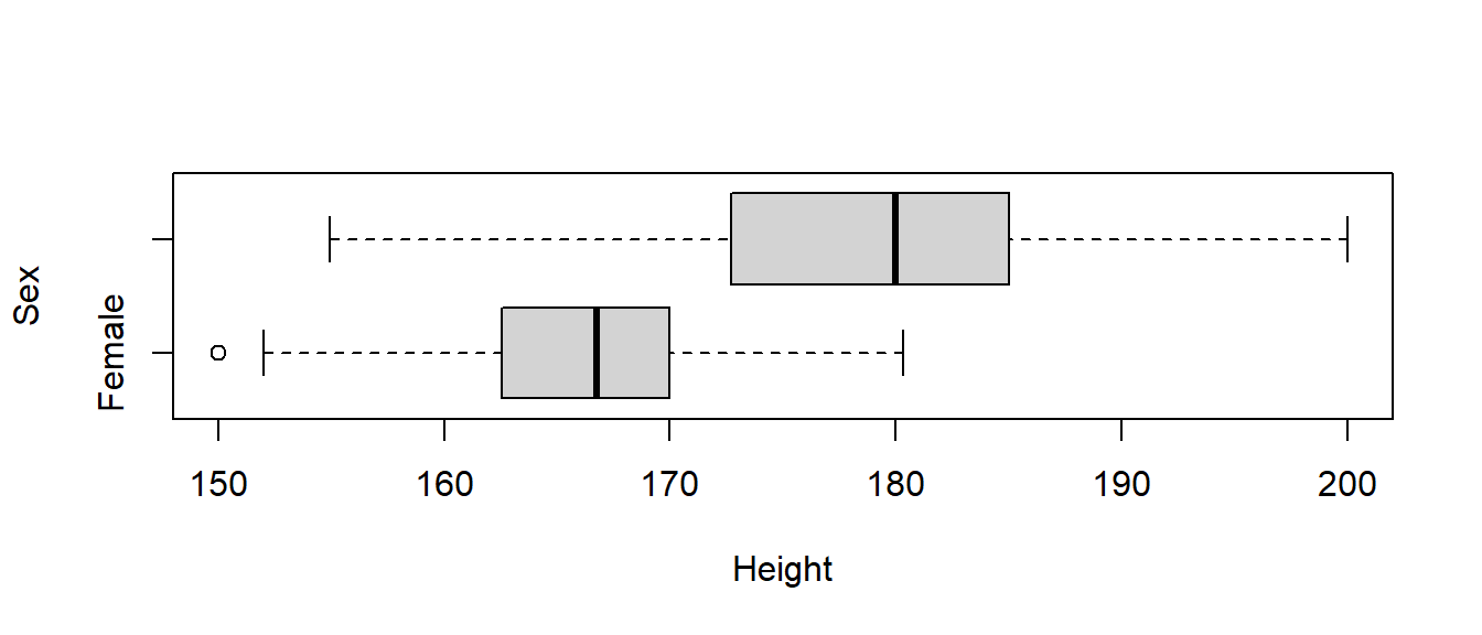
##
##  Welch Two Sample t-test
##
## data:  Height by Sex
## t = -12.924, df = 192.7, p-value < 2.2e-16
## alternative hypothesis: true difference in means between group Female and group Male is not equal to 0
## 95 percent confidence interval:
##  -15.14454 -11.13420
## sample estimates:
## mean in group Female   mean in group Male
## 165.6867 178.8260##
## Two Sample t-test
##
## data: Height by Sex
## t = -12.85, df = 206, p-value < 2.2e-16
## alternative hypothesis: true difference in means between group Female and group Male is not equal to 0
## 95 percent confidence interval:
## -15.15536 -11.12338
## sample estimates:
## mean in group Female mean in group Male
## 165.6867 178.8260Finally, just a bit of code to show how a paired samples \(t\)-test (on DEPENDENT samples) is equivalent to a single sample \(t\)-test on the differences. This test looks at the difference between the span of one’s writing hand versus non-writing hand.
##   min   Q1 median  Q3 max       mean       sd   n missing
##  -1.6 -0.3      0 0.5 4.7 0.08644068 0.624386 236       1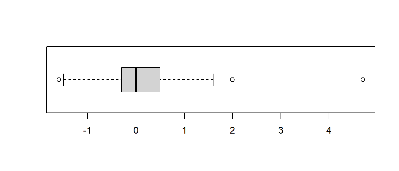
##
##  Paired t-test
##
## data:  survey$Wr.Hnd and survey$NW.Hnd
## t = 2.1268, df = 235, p-value = 0.03448
## alternative hypothesis: true mean difference is not equal to 0
## 95 percent confidence interval:
##  0.006367389 0.166513967
## sample estimates:
## mean difference
## 0.08644068##
## One Sample t-test
##
## data: survey$Diff
## t = 2.1268, df = 235, p-value = 0.03448
## alternative hypothesis: true mean is not equal to 0
## 95 percent confidence interval:
## 0.006367389 0.166513967
## sample estimates:
## mean of x
## 0.08644068