Chapter 1 Probability

These notes are meant to supplement, not replace your textbook. I will occasionally cover topics not in your textbook, and I will stress those topics I feel are most important.

Let’s start with an informal notion of probability, where we try to assign a numerical percentage or proportion or fraction to something happening. For example, you might be interested in the chance that it will rain tomorrow. How would you go about assigning a numerical value to this event?

This would be an example of the subjective approach to probability, based on an event that cannot be repeated, although a weather forecaster might run many simulations of a weather model (which would be closer to the objective approach). Another example of the subjective approach would be assigning a percentage chance of your favorite NFL team winning the next Super Bowl.

Some of the flaws of the subjective approach to probability could include bias (you might assign your favorite team a higher percentage chance of winning than the team should have because it is an event you would like to have happen, or vice versa for a rival team you do not like) or knowledge/lack of knowledge of the person assigning the probability (maybe you know little to nothing about the NFL).

We will typically prefer the objective approach to probability instead. When we assign a numerical value to the probability of an event that CAN be repeated, we obtain an objective probability.

As the simplest type of experiment that can be repeated, consider flipping a coin, where event $H$ is the probability of obtaining ‘heads’. I know you already know the answer to the question ‘What is $P(H)$?’, but suppose you are a Martian and have never encountered this strange object called a ‘coin’ before.

Our friendly Martian decides to conduct a simulation to determine $P(H)$ by flipping the coin a large number of times. Suppose the Martian flips the coin 10,000 times and obtains 5,024 heads. His estimate of the probability is \[ \begin{aligned} P(H) & = \frac{\text{number of occurrences of event}}{\text{total number of trials}} \\ P(H) & = \frac{5024}{10000} = 0.5024 \\ \end{aligned} \]

This is called the empirical or the relative frequency approach to probability. It is useful when the experiment can be simulated many, many times, especially when the mathematics for computing the exact probability is difficult or impossible.

The mathematician John Kerrich actually performed such an experiment when he was being held as a prisoner during World War II.

This example illustrates the Law of Large Numbers, where the relative frequency probability will get closer and closer to the true theoretical probability as the number of trials increase.

For instance, if I flipped a coin ten times and got 6 heads, you probably wouldn’t think anything was unusual, but if I flipped it 10,000 times and got heads 6,000 times, you would question the assumption that the coin was “fair” and the outcomes (heads or tails) were equally likely.

The other type of objective probability is called classical probability, where we use mathematics to compute the exact probability without actually performing the experiment.

For example, we can determine $P(H)$ without ever flipping a coin. We know there are two possible outcomes (heads and tails). If we are willing to assume the probability of each outcome is equally likely (i.e. a “fair” coin), then $P(H)=\frac{1}{2}$.

Similarly, if we roll a single 6-sided die and let event $A$ be the event that the die is less than 5, then notice that 4 of the 6 equally likely events contain our desired outcome, so $P(A)=\frac{4}{6}$.

Clever mathematics, which can get quite difficult, can be used to compute probabilities of events such as the probability of getting a certain type of hand in a poker game or winning the jackpot in a lottery game such as Powerball.

A standard deck of cards contains 52 cards. The cards are divided into 4 suits (spades, hearts, diamonds, clubs), where the spades and clubs are traditionally black and the hearts and diamonds are red. The deck is also divided into 13 ranks (2, 3, 4, 5, 6, 7, 8, 9, 10, Jack, Queen, King, Ace). The Jack, Queen, King are traditionally called face cards. The Ace can count as the highest and/or lowest ranking card, depending on the particular card game being played.

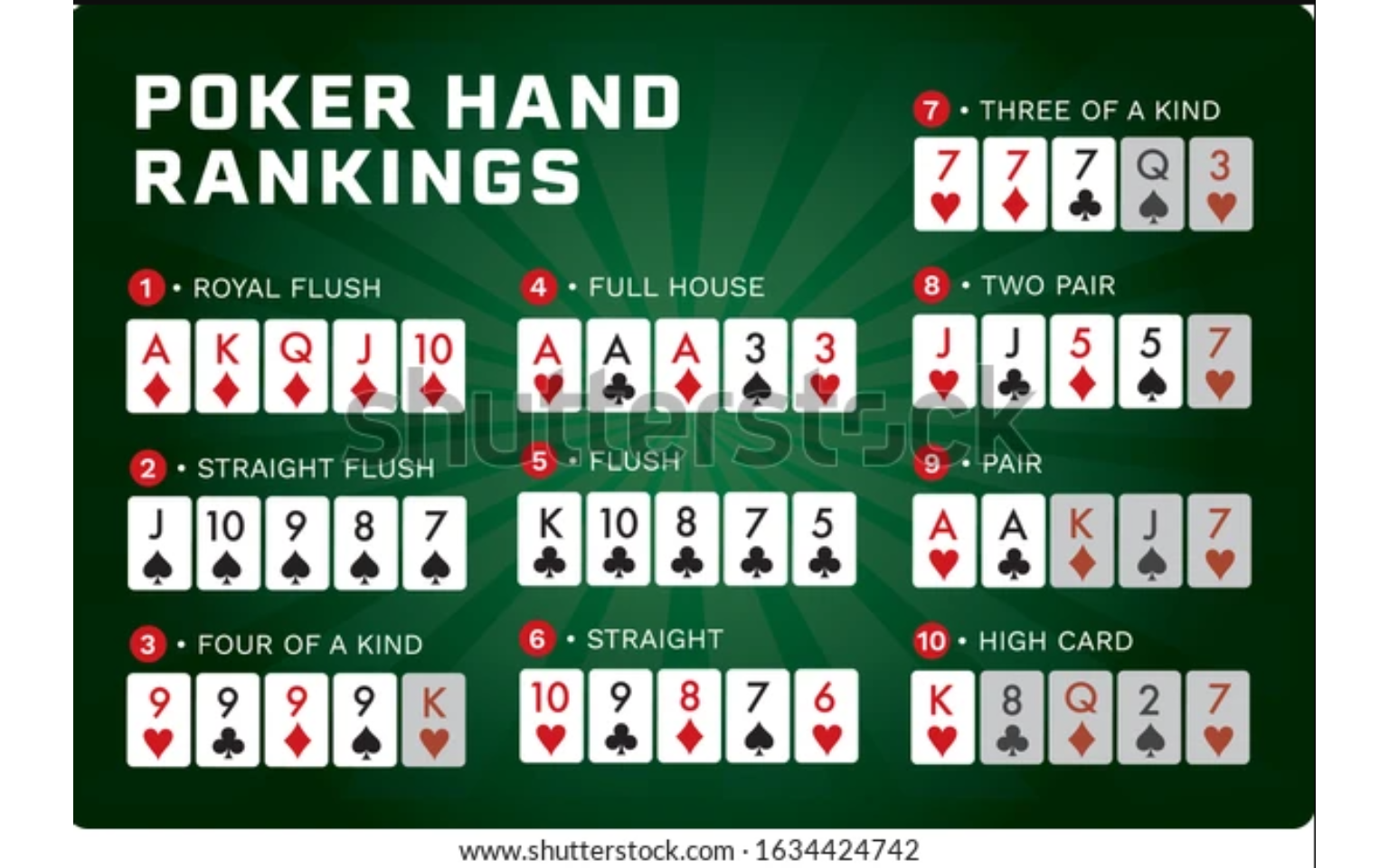
The popular card game poker can be played in many ways–the variation known as “Texas holdem” is currently the most popular. Most poker variations are based on ranking ones best 5 card hand, where the hand that is the hardest to get (i.e. has the lowest probability of occuring) is the winner.

A graph of the hands, from the strongest (royal flush, almost impossible to get), to the weakest (high card) is on the next page. Notice a “flush” (all cards same suit) beats a “straight”” (all cards in sequence or “order”) and that both of these hands beat a “three of a kind”.

Suppose in a game of Texas Holdem that we have been dealt the Ace of Hearts and the King of Hearts. The opponent has been dealt the Ace of Diamonds and the Queen of Diamonds.

The flop and turn have been dealt and the players are “all-in”, so 4 of the 5 community cards are known and only the “river” (the last community card) is unknown. Suppose the known cards are the Queen of Hearts, Ten of Diamonds, Seven of Clubs, and Five of Hearts. What is your probability of winning once the last card is revealed? Currently, you are losing, as you have no pair but the opponent has a pair of quuens.

First, let’s figure out how many unknown cards are left. You have seen the 2 cards in your hand, the 2 cards in the opponent’s hand, and the 4 cards on the board, so 52-8=44 cards are unknown.

Next, consider cards that will make us a hand that will make us a winning hand. If the last card is a heart, we will make an ace-high flush and will win. There are 13-4=9 hearts left that will make a winning flush.

A Jack will make a straight (we would have AKQJ10), and there are 4 jacks left in the deck. Of course, one of them is the Jack of Hearts, so there are 3 non-heart Jacks left that makes a winning straight.

What if the last card is an Ace? There are two aces left, but even though we would improve to a pair of aces, the opponent improves to two pair (Aces and Queens), and we still lose.

If the last card is one of the three remaining kings, we improve to a pair of kings, which would beat our opponent’s pair of queens.

Thus, our chance of winning is $\frac{9+3+3}{52-2-2-4}=\frac{15}{44}$, or about 34%. This is an example of the classical approach to probability, where we used mathematics to compute our chance of winning without simulating the experiment. One could have also done a simulation by writing computer code to play out this hand thousands of times, or manually by actually dealing out cards in this situation many times, to use the relative frequency approach.

Let’s formalize this by looking at some defintions and basic set theory.

1.1 Properties of Probability

A random experiment is a situation where the outcome cannot be predicted with certainty. Examples we’ve already considered include the probability of flipping a coin and getting heads, the chance of rain tomorrow, or the outcome of a hand of Texas Holdem poker.

An outcome or element is a possible result of an experiment.

An event is a set of one or more possible outcomes. We will typically denote events with capital letters from the beginning of the alphabet. The sample space is all possible outcomes, which we denote as $S$. An event $A$ will be a subset of space $S$, $A \subset S$. In general $A_1 \subset A_2$ if every event in $A_1$ is also in $A_2$.

A player receives one card, at random, from the deck. Let $A$ be the event the card is an Ace, $B$ that the card is a heart, and $C$ that the card is a face card (Kings, Queens, Jacks). The space $S$ here consists of all 52 cards in the deck. $A$, $B$, and $C$ are all subsets of $S$.

\[P(A)=\frac{4}{52}=\frac{1}{13}\]

\[P(B)=\frac{13}{52}=\frac{1}{4}\]

\[P(C)=\frac{4+4+4}{52}=\frac{12}{52}\]

The union of two sets consists of all elements that are in at least one of the sets. This is denoted as $A \: or \: B$ or $A \cup B$.

The intersection of two sets consists of all elements that are in both sets. This is denoted as $A \: and \: B$ or $A \cap B$.

(will show in class with Venn Diagrams)

In the cards example, the union of $A$ and $B$ consists of the set of all 4 aces and all 13 hearts. The intersection of $A$ and $B$ consists of the set with a single element, the Ace of Hearts which is the only card that belongs to both set $A$ and set $B$. Since the Ace of Hearts, is in both sets, there are actually only 16 elements, not 17, in $A \cup B$.

\[P(A \cup B)= P(A) + P(B) - P(A \cap B) =\frac{4}{52}+\frac{13}{52}-\frac{1}{52}=\frac{16}{52}\] This is called the Addition Rule. We’ll formally define the set function $P$ shortly–it’s the “probability” of an event.

If we consider events $A$ and $B$ instead, the union of $A$ and $C$ contains the 4 aces and the 12 face cards, for a total of 16 cards. Unlike the previous example, this time there are no elements in common between the two sets, so the intersection of $A$ and $C$ is the null set or empty set $\emptyset$.

\[P(A \cap C)=\frac{0}{52}=0\] \[P(A \cup C)=\frac{4}{52}+\frac{12}{52}-\frac{0}{52}=\frac{16}{52}\]

Here, the circles in the Venn diagram representing $A$ and $C$ will NOT overlap each other.

The complement of an event, denoted as $A'$ or $A^c$, consists of all elements in space $S$ that are NOT in set $A$. Here, $A'$ represents all cards that are not aces, which would be the 48 non-aces in the deck.

\[P(\: not \: A) = P(A')=1-P(A)=1-\frac{4}{52}=\frac{48}{52}\]

This result is known as the Complement Rule. This may seem trivial for this example, but the Complement Rule is very helpful in situations where finding the probability of $A$ is difficult or impossible but finding the probability of $A'$ is easier.

Mutually exclusive events $A_1,A_2,\cdots,A_k$ means that $A_i \cap A_j = \emptyset, i \neq j$. These are disjoint sets. An example would be sets $A_1$ (aces), $A_2$ (deuces), $A_3$ (treys) in a deck of cards.

Exhaustive events $A_1,A_2,\cdots,A_k$ means that $A_1 \cup A_2 \cup \cdots \cup A_k=S$. An example would be sets $A_1$ (hearts), $A_2$ (diamonds), $A_3$ (face cards), and $A_4$ (black cards). Notice that not all of these sets are mutually exclusive; while $A_1 \cup A_2 = \emptyset$, $A_1 \cup A_3$ would not be the empty set but would consist of 3 cards (the king/queen/jack of hearts).

An example where the four sets are the four suits: $A_1$ (hearts), $A_2$ (diamonds), $A_3$ (spades), $A_4$ (clubs) are mutually exclusive and exhaustive, combining both properties.

The algebrea of set operations follow these laws: (will do some Venn diagrams as informal “proofs”)

Commutative Laws \[A \cup B = B \cup A\] \[A \cap B = B \cap A\]
Associative Laws \[(A \cup B) \cup C = A \cup (B \cup C)\] \[(A \cap B) \cap C = A \cap (B \cap C)\]
Distributive Laws \[ A \cap (B \cup C) = (A \cap B) \cup (A \cap C)\] \[ A \cup (B \cap C) = (A \cup B) \cap (A \cup C)\]
De Morgan’s Laws \[(A \cup B)' = A' \cap B'\] \[(A \cap B)' = A' \cup B'\]

Suppose I have three coins, each of which I flip, and I want to know the probability of obtaining heads on at least one of three flips. If you don’t know how to calculate this probability, you could conduct the experiment many times. I wrote a small computer program that simulated doing this experiment 1000 times. We will assume the coin is fair (i.e. probability of heads is 0.5).

## x
##   0   1   2   3 
## 123 362 379 136

Let event $A$ be the event of obtaining heads on at least one coin toss and $\mathcal{N}(A)$ be the count of how many times $A$ occured. Here, $\mathcal{N}(A)=362+379+136=877$ and the relative frequency probability is $P(A)=\frac{\mathcal{N}(A)}{n}=\frac{877}{1000}=0.877$. It turns out that the classical probability of event $A$ is $P(A)=1-(0.5)^3=0.875$.

A set function is a function that maps set to real numbers. In the above example, we would like to associate event $A$ with a number $P(A)$ such that the relative frequency $\frac{\mathcal{N}(A)}{n}$ stabilizes with large $n$–the function $P(A)$ is such a function.

Probability is a real-valued set function $P$ that assign to each event $A$ in sample space $S$ a numerical value $P(A)$ that satisfies the following:

$P(A) \geq 0 \: \forall A \in S$
$P(S)=1$
If $A_1, A_2, A_3, \cdots$ are events and $A_i \cap A_j = \emptyset, i \neq j$, then \[P(A_1 \cup A_2 \cup \cdots \cup A_k)=P(A_1) + P(A_2) + \cdots + P(A_k)\] for each positive integer $k$ and \[P(A_1) \cup A_2 \cup A_3 \cup \cdots)=P(A_1)+P(A_2)+P(A_3)+\cdots\] for a countably infinite number of events.

An example of the latter is if we were calculating how many flips of a coin were needed to obtain the first heads. We might need 1 flip, 2 flips, 3 flips, etc. Theoretically, we might flip tails thousands or millions of times before getting the first heads.

Let’s prove some basic theorems for some of the fundamental concepts of probability.

Complement Rule (Theorem 1.1-1) For any event $A \in S$, $P(A)=1-P(A')$.

Proof: \[S = A \cup A'\] \[A \cap A' = \emptyset\] \[\text{Therefore } P(A \cup A') = 1\] \[P(A) + P(A') =1\] \[P(A)=1-P(A')\]

A famous application of the Complement Rule to compute a difficult probability is the so-called Birthday Problem. How many people do we need to have in a room for there to be a 50% chance or more of having at least one pair of people with matching birthdays?

(make a guess)

Solution: It’s too hard to compute the probability of at least one birthday match, which is our desired event $A$. It is easier to compute the probability of no birthday match, $A'$. We will make the simplying assumptions that all 365 birthdays are equally likely and that leap years do not exist.

If $n=2$, then $P(A')=\frac{364}{365}\approx 0.997$, so $P(A)=1-0.997=0.003$

If $n=3$, then $P(A')=\frac{364}{365} \times \frac{363}{365} \approx 0.992$, so $P(A)=1-0.992=.008$

and so forth…

With $n=23, $P(A')=\frac{364}{365}\times\frac{363}{365}\times \cdots \times \frac{343}{365} \approx 0.493$, so $P(A')=1-0.493=0.507$. This is when the probability of a birthday match first exceeds 50% and this number is much lower than most people guess off the top of their head.

https://en.wikipedia.org/wiki/Birthday_problem

Theorem 1.1-2: $P(\emptyset)=0$

Proof: Let $A=\emptyset$.

Then $A'=S$.

Since $P(A)=1-P(A')$, then $P(\emptyset)= 1-P(S)=1-1=0$.

Theorem 1.1-3: If events $A$ and $B$ are such that $A \subset B$, then $P(A) \leq P(B)$.

Proof: Notice that $B=A \cup (B \cap A')$ and $A \cap (B \cap A')=\emptyset$.

Hence, $P(B)=P(A)+P(B \cap A') \geq P(A)$ since $P(B \cap A') \geq 0$.

Theorem 1.1-4: For each event $A$, $P(A) \leq 1$.

Proof: Since $A \subset S$, then $P(A) \leq P(S)$ and hence $P(A) \leq 1$.

**Additon Rule: Theorem 1.1-5 If $A$ and $B$ are any two events, then $P(A \cup B) = P(A) + P(B) - P(A \cap B)$.

Proof: Note that $A \cup B = A \cup (A' \cap B)$ (a union of mutually exclusive events)

So $P(A \cup B)=P(A) + P(A' \cap B)$.

Also, $B = (A \cap B) \cup (A ' \cap B)$ (also a union of mutually exclusive events).

Thus, $P(B) = P(A \cap B) + P(A' \cap B)$.

So $P(A' \cap B) = P(B) - P(A \cap B)$.

By substitution, $P(A \cup B) = P(A) + P(B) - P(A \cap B)$.

Theorem 1-1.6: If $A$, $B$, and $C$ are any three events, then \[P(A \cup B \cup C)=P(A)+P(B)+P(C)-P(A \cap B)-P(A \cap C)- P(B \cap C) + P(A \cap B \cap C)\]

Hint: Write $A \cup B \cup C = A \cup (B \cup C)$ and apply Theorem 1.1-5.

This is known as the inclusion-exclusion principle–the idea is that the over-generous inclusion needs to be corrected for with exclusion. With two events, when we add together the probability of events $A$ and $B$, we include too much when $A$ and $B$ have a non-empty intersection, such as when $A$ is the set of aces and $B$ is the set of hearts. We included the ace of hearts twice, and thus apply a correction by excluding the probability of the intersection $A \cap B$. Notice for three events, we exclude all two way intersections, but that is an over-correction and we have to add the three-way intersection back in. You might informally “prove” this with a Venn diagram.

1.2 Methods of Enumeration

Multiplication Rule (or the $mn$-rule)

Suppose we have 2 independent events. $A$: roll a die (6 outcomes) $m=6$ $B$: flip a coin (2 outcomes) $n=2$

$m \times n = 6 \times 2=12$ outcomes of the two events

\[S=\{1H,2H,3H,4H,5H,6H,1T,2T,3T,4T,5T,6T\}\]

A tree diagram could be used to visualize this.

Another example: Suppose you go to a banquet where there are 4 choices for the main course (steak, chicken, fish, vegetarian) and 5 choices for beverage (water, coffee, iced tea, cola, diet cola).

There would be $4 \times 5=20$ possible selections of a main course and beverage. Of course, the number of selections could be reduced due to dietary restrictions. I have a friend who is a pescatarian and would only choose from the fish and vegetarian choices, so they would have $2 \times 5=10$ possible selections.

We could, of course, extend to 3 or more events. If there were two desserts available (cheesecake, ice cream), then there would be $4 \times 5 \times 2=40$ possible meal selections.

Now suppose we have a set $A$ with $n$ elements. For example, imagine a mathematics & statistics department with $n=20$ professors. Suppose we take $r$-tuples that are elements of set $A$. If $r=3$, this means to choose three members of the set. For instance, we might have a 3-tuple that consists of three members of this department: (Dr. Luck, Dr. Chance, Dr. Gamble).

There would be $n!$ arrangements of the 20 elements of this set, assuming order matters. In this case, $20!$ is a very large number, about $2.4 \times 10^18$. Each of these arrangments is called a permutation of the $n$ objects.

As a smaller example, take the name CHRIS, which consists of $n=5$ letters. There are $5!=120$ permutations of the letters of this name. Of course, most of them are nonsense that do not form real words, such as RSCIH.

If we are selecting exactly $r$ objects from $n$ different objects, with $r \leq n$, the number of possible such arrangements is:

\[_nP_r = P_r^n = n \times n-1 \times n-2 \times \cdots \times n-r+1\] This expression could be written:

\[P_r^n = \frac{n(n-1)(n-2)\cdots(n-r+1)(n-r)\cdots(3)(2)(1)}{(n-r)\cdots(3)(2)(1)} = \frac{n!}{(n-r)!}\]

Each of the $P_r^n$ arrangements (ordered subsets) is called a permutation of $n$ objects taken $r$ at a time.

Suppose that $r=3$ of the $n=20$ professors are getting raises this year, where the size of the raise is $5000, $1000, and $10. Clearly, order matters.

There are $P_3^{20}=\frac{20!}{(20-3)!}=20 \times 19 \times 18=6840$ such permutations. One such permutation is (Dr. Mecklin, Dr. Pathak, Dr. Williams) where since I was selected first, I get the $5000 raise. Another such permutation is (Dr. Roach, Dr. Donovan, Dr. Mecklin) where I get the $10 raise. Clearly order is important! I strongly prefer the first permutation!

This is an example of sampling without replacement, where once a professor was selected, they would not be chosen again (such as if names were drawn out of a hat). Card games such as poker typically feature sampling without replacement.

Sampling with replacement occurs when an object is selected and then replaced in the set, so it can be selected again. Dice rolling is a common example of this. If we roll a standard six-sided die twice, we could get a roll of 2 on both the first and second roll, whereas if you were dealt 2 cards from a deck of 52 and the first card was the 10 of hearts, the second card will NOT be the 10 of hearts.
Often the order of selection is not important. In my example with raises for professors, suppose that the $r=3$ professors selected will all receive a $1000 raise, so that being selected first, second, or third is unimportant. Now there is no difference between the subsets (Dr. Mecklin, Dr. Williams, Dr. Pathak) versus (Dr. Williams, Dr. Pathak, Dr. Mecklin).
When playing a card game such as Texas holdem poker, if your hand is the Ace of hearts and King of hearts, it is unimportant whether the Ace was the first or second card dealt to you.
We can compute the number of unordered subsets of $n$ objects taken $r$ at a time: these are referred to as combinations or the binomial coefficient.
\[_rC_n=C_r^n=\binom{n}{r}=\frac{n!}{r!(n-r)!}\]
Notice that $C_3^{20}=\frac{20!}{3!17!}=1140$ combinations of 20 professor chosen 3 at a time. Notice this is $\frac{1}{3!}=\frac{1}{6}$ of the number of permutations, as there are $r!=3!=6$ different ways I could arrange $r=3$ names.
The name binomial coefficient comes from the fact that this expression arises in the expansion of a binomial term.
\[(a+b)^n = \sum_{r=0}^n \binom{n}{r}b^r a^{n-r}\] If $n=4$, then: \[(a+b)^4 = \binom{4}{0}b^0 a^4 + \binom{4}{1}b^1 a^3 + \binom{4}{2}b^2 a^2 + \binom{4}{3}b^3 a + \binom{4}{4}b^4 a^0\] \[(a+b)^4 = a^4 + 4 a^3b + 6 a^2 b^2 + 4 ab^3 + b^4\]

Combinations are very useful in computing the probability of certain poker hands. Brian Alspach, a retired Canadiam mathematics professor, has probably more than you ever wanted to know about the combinatorics of various poker hands: http://people.math.sfu.ca/~alspach/computations.html

Here, we will deal a $r=5$ card hand without replacement from the standard deck of $n=52$ cards.

Let event $A_1$ be getting any two pair. This means that we get 2 cards of one rank, 2 cards from a second rank, and a singleton from one of the 11 remaining ranks. For example, I might get the 2 of clubs, 2 of spades, 6 of diamonds, 6 of spades, and the 9 of hearts.

The probability of such a hand is:

\[P(A_1)=\frac{\binom{13}{2}\binom{4}{2}\binom{4}{2}\binom{11}{1}\binom{4}{1}}{\binom{52}{5}}=\frac{123,552}{2,598,960}=0.0475\] The $\binom{52}{5}$ combination term in the denominator is the number of possible $5$-tuples (i.e. poker hands) that could be dealt from the set of $n=52$ cards.

The order is not important (for example, it doesn’t matter if you received the 9 of hearts as the first card, last card, or any other position). There would be many many more possible permutations of 5 cards from 52.

\[P_5^{52}=\frac{52!}{47!}=311,875,200\]

Another correct way to compute the probability of two pair would be to select the rank of the singleton first, rather than last.

\[P(A_1)=\frac{\binom{13}{1}\binom{4}{1}\binom{12}{2}\binom{4}{2}\binom{4}{2}}{\binom{52}{5}} = \frac{123,552}{2,598,960}=0.0475\]

Notice that $\binom{13}{2}\binom{11}{1}=78 \times 11 = 858$ (from selecting the ranks of the pairs first) and $\binom{13}{1}\binom{12}{2}= 13 \times 66 = 858$ (from selecting the rank of the singleton first).

A common mistake is the following:

\[P(A_1)=\frac{\binom{13}{1}\binom{4}{2}\binom{12}{1}\binom{4}{2}\binom{11}{1}\binom{4}{1}}{\binom{52}{5}}\]

Notice that $\binom{13}{1}\binom{12}{1}= 13 \times 12 =156$, which is twice as large as $\binom{13}{2}=78$, and thus the probability computed would be twice as large as it should be. When we selecting the ranks of the pairs one at a time, then a hands like deuces & sixes is counted separtely from sixes & deuces, although in poker this order does not matter.

Let $A_2$ be a full house (i.e. a three of a kind and a pair, such as 3 kings and 2 sevens).

\[P(A_2)=\frac{\binom{13}{1}\binom{4}{3}\binom{12}{1}\binom{4}{2}}{\binom{52}{5}}=\frac{3,744}{2,598,960}=.0014\]

Why would using $\binom{13}{2}\binom{4}{3}\binom{4}{2}$ as the numerator be wrong? Because in selecting the ranks of the three of a kind and the pair at the same time, this fails to distinguish between the hand KKK77 and 777KK.

Let $A_3$ be the probability that all 5 cards are the same suit. Note that this will include flushes, straight flushes, and royal flushes as our calculations will not take into consideration the possibility that the 5 cards are all in sequence and thus make a straight. Refer to Dr. Alspach’s website for how to deal with straights and straight flushes. http://people.math.sfu.ca/~alspach/comp18/

\[P(A_3)=\frac{\binom{4}{1}\binom{13}{5}}{\binom{52}{5}}=\frac{5,148}{2,598,960}=0.00198\]

1.3 Conditional Probability

Conditional probability is defined to be the probability of an event $B$ occuring, if (or given) that another event $A$ has occurred.

\[P(B|A) = \frac{P(A \cap B)}{P(A)}, P(A)>0\]

where: (1) $P(B|A) \geq 0$ and $P(A|A)=1$.

Example: Apples/Bananas

Suppose it is known that in a population of school children that $P(A)=0.8$, $P(B)=0.7$, and $P(A \cap B)=0.6$ (the intersection joint probability of the two events)

As review, the probability of the union of $A$ and $B$ is: \[P(A \cup B) = P(A) + P(B) - P(A \cap B) = 0.8 + 0.7 - 0.6 = 0.9\]

This can be interpreted as that 90% of children like at least one of the two fruits.

\[P(A \cup B)' = 1 - P(A \cup B)=1-.9=.1\]

This can be interpreted as that 10% of the children like neither of the two fruits. We could have expressed with De Morgan’s Law.

\[P(A \cup B)' = P(A' \cap B')\]

Note that \[P(A \cap B') = P(A)-P(A \cap B)=0.8-0.6=0.2\] the 20% of children that like apples but not bananas. Similarly, \[P(A` \cap B) = P(B)-P(A \cap B)=0.7-0.6=0.1\] the 10% of children that like bananas but not apples.

The conditional probability of a child liking bananas if/given that they like apples is \[P(B|A)=\frac{P(B \cap A)}{P(A)}=\frac{0.6}{0.8}=0.75\]

Notice that $P(B|A) \neq P(B)$. In this situation, the conditional probability is greater, which here means that children are more likely to like bananas if they also like apples. The probability of event $B$ was dependent on the event $A$.

In the special case where $P(B|A)=P(A)$, the two events are said to be independent and we will focus on this situation in the next section. In this case, the probability of the intersection of two events (the joint probability) is \[P(A \cap B)=P(A)P(B)\]

In general, finding the probability of an intersection requires knowing the conditional probability of the two events. A very common mistake is to try to find the probabilities of all intersections by multiplication of the probabilities of the individual events without taking dependence into consideration.

Multiplication Rule: \[P(A \cap B) = P(A)P(B|A) = P(B)=P(A|B)\]

Dice example

Suppose we roll a standard six-sided die and a standard four-sided die. We could construct the sample space as a $6 \times 4$ grid of dots, with the 6 rows representing the results $1,2,3,4,5,6$ obtained on the six-sided die and the 4 columns the results $1,2,3,4$ from the four-sided die, giving us $6 \times 4 = 24$ combinations of die rolls that are equally likely. Of course, some of the sums will be the same with different rolls and are NOT equally likely; for instance, we get a sum of 4 by rolling a 1 then a 3, a 2 then another 2, or a 3 then a 1.

Suppose we want to know the probability that the sum will be equal to 8 if the first die is a 5. Here, $P(A)$ is the probability of getting a 5 on the first roll, which is $P(A)=1/6$. The probability of the intersection $A \cap B$ (getting a total of 8 if the first die was a 5) is $P(A \cap B)=1/24$, as this happens if we then roll a 3 on the four-sided die, which is one of the 24 equally likely outcomes of the two rolls.

So the conditional probability of getting a sum of 8 if we got a 5 with the first roll is: \[P(B|A)=\frac{P(A \cap B)}{P(A)}=frac{1/24}{1/6}=\frac{6}{24}=\frac{1}{4}\]

Notice this is greater than $P(B)$, the probability of getting a sum of eight, which happens with the outcomes (62,53,44). \[P(B)=\frac{3}{24}=\frac{1}{8}\]

It should seem reasonable that our probability of a large total such as 8 increases if we get a large result on the first die. There are certain results (getting a 1, 2, or 3 with the six-sided die) that would make getting a total of 8 impossible, where $P(B|A)=0$.

Poker example: In Texas Holdem poker, a hand starts with each player being dealt two cards face down. The best starting hand in the game is a pair of Aces, which is referred to as pocket Aces.

Suppose that $A_1$ is the first card dealt to you, and you peek at it before the dealer deals you the second card, event $A_2$. A pair of Aces (pocket aces) is the intersection $A_1 \cap A_2$, and the union of the events $A_1 \cup A_2$ is when you get at least one Ace in your hand.

The probability that the first card is an Ace, when you peek, is $P(A_1)=\frac{4}{52}=\frac{1}{13}$. Why would it be incorrect to say the probability of pocket aces is \[P(A_1 \cap A_2)=\frac{1}{13 }\times \frac{1}{13}=\frac{1}{169}\]

That is incorrect because that would assume sampling with replacement, where after receiving and looking at the first card, it was shuffled back into the deck. This, of course, is not the way poker or other card games are played. Instead sampling without replacement is used and the second card is dealt from the remaining cards, with 51 cards unknown to you. Events $A_1$ and $A_2$ are NOT independent.

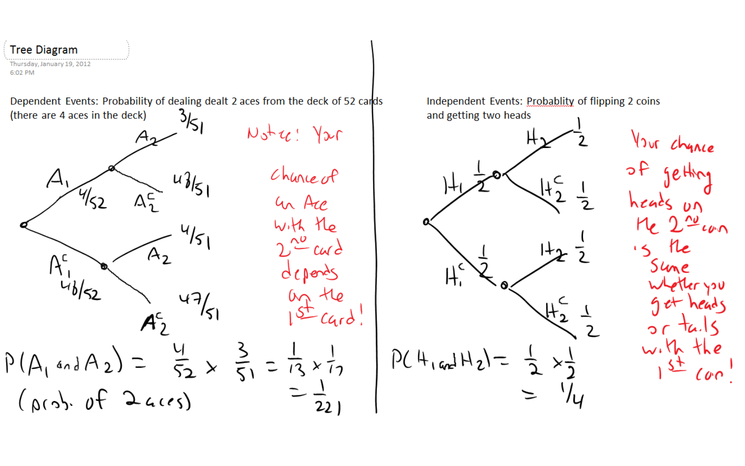
I will draw a tree diagram to picture the four possibilities. Note the conditional probabilities for the second card are: $P(A_2|A_1)=3/51$ (i.e. 3 aces left in the deck when the first card is an ace), $P(A_2'|A_1)=48/51$ (i.e. 48 non-aces left in the deck when the first card is an ace), $P(A_2|A_1')=4/51$ (i.e. still 4 aces left in the deck if the first card is not an ace), and $P(A_2'|A_1')=47/51$ (i.e. 47 non-aces left in the deck if the first card is not an ace).

\[P(A_1 \cap A_2)=\frac{4}{52}\times\frac{3}{51}=\frac{1}{221}\]

\[P(A_1 \cap A_2')=\frac{4}{52}\times\frac{48}{51}=\frac{16}{221}\]

\[P(A_1') \cap A_2)=\frac{48}{52}\times\frac{4}{51}=\frac{16}{221}\]

\[P(A_1' \cap A_2')=\frac{48}{52}\times\frac{47}{51}=\frac{188}{221}\]

The probability of exactly one ace in the hand is $\frac{16+16}{221}=\frac{32}{221}$.

1.4 Independent Events

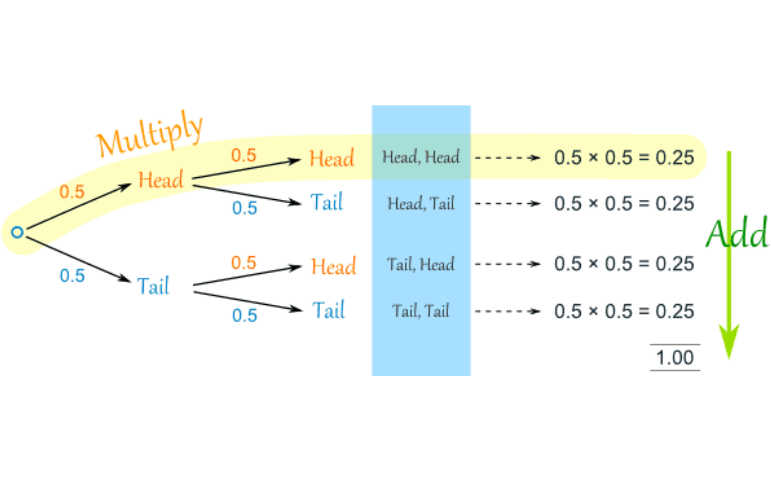
If the probability of event $B$ is unchanged by whether or not event $A$ happened, the events are said to be independent. A trivial example is the result of two tosses of a coin. I’ll draw a tree diagram to show those, and notice that the second level of branches (with the conditional probabilities) will have the same probabilities whether the first event happened or not. Unlike the Texas Holdem situation, where your probability of being dealt an ace with the second hand depends on the first card (and changes based on what that first card is), the chance of getting heads or tails with the second coin toss is unaffected and does not depend on the first toss.

\[P(H_1 \cap H_2)=\frac{1}{2}\times\frac{1}{2}=\frac{1}{4}\] \[P(H_1 \cap T_2)=\frac{1}{2}\times\frac{1}{2}=\frac{1}{4}\] \[P(T_1 \cap H_2)=\frac{1}{2}\times\frac{1}{2}=\frac{1}{4}\] \[P(T_2 \cap T_2)=\frac{1}{2}\times\frac{1}{2}=\frac{1}{4}\]

Definition: Events $A$ and $B$ are independent iff (if and only if) \[P(A \cap B)=P(A)P(B)\]

Theorem 1.4-1: If $A$ and $B$ are independent events, then the following pairs of events are also independent: (a) $A$ and $B'$; (b) $A'$ and $B$; and (c) $A'$ and $B'$

Proof of part (a): By the axioms of a probability function, we know that if $P(A)>0, then $P(B'|A)=1-P(B|A)$. Thus:

\[P(A \cap B')=P(A)P(B'|A)=P(A)[1-P(B|A)]=P(A)[1-P(B)]=P(A)P(B')\]

since by hypothesis $A$ and $B$ are independent and $P(B|A)=P(B)$. So, $A$ and $B'$ are independent events.

Proofs for parts (b) and (c) are quite similar.

Definition: Events $A$,$B$, and $C$ are mutually independent iff:

$A$, $B$, and $C$ are pairwise independent, that is: \[P(A \cap B)=P(A)P(B), P(A \cap C)=P(A)P(C), P(B \cap C)=P(B)P(C)\]
$P(A \cap B \cap C)=P(A)P(B)P(C)$

Example: Suppose a hockey game has gone to a penalty shootout, where three players from each team are selected to take the penalty shot. Suppose the players taking the shots for the Nashville Predators are denoted $A$, $B$, and $C$, where we pretend that these events are mutually independent and are unaffected by whether other players on the Predators or the opposition make or miss their shots. If $P(A)=0.4$, $P(B)=0.5$ and $P(C)=0.6$, what is the probability of making all three shots? Missing all three shots?

Making all three shots would be \[P(A)\cap P(B) \cap P(C)=(0.4)(0.5)(0.6)=0.12\] Missing all three shots would be \[P(A' \cap B' \cap C')=(1-0.4)(1-0.5)(1-0.6)=0.12\]

I could draw a tree diagram to illustrate all possibilities, including when the team makes exactly 1 or exactly 2 shots.

1.5 Bayes Theorem

This famous theorem, due to the 18th century Scottish minister Reverend Thomas Bayes, is used to solve a particular type of ‘inverse probability’ problems.

The usual way of stating Bayes’ Theorem, when there are only two possible values, or states, for event $B$, is: \[P(B|A)=\frac{P(A|B) \times P(B)}{P(A|B) \times P(B) + P(A|B^c) \times P(B^c)}\]

where $P(B)$ is called the probability of the event and the final answer, $P(B|A)$ is the or revised probability based on information from event $A$.

If the space $S$ is partitioned into $k$ mutually exclusive events $B_1 \cup B_2 \cup \cdots \cup B_k =S$ where $B_i \cap B_j = \emptyset, i \neq j$, then Bayes Theorem generalizes into:

\[P(B_k|A)=\frac{P(B_k) P(A|B_k)}{\sum_{i=1}^m P(B_i)P(A|B_i)}\]

Bayes’ Theorem is often used in medicine to compute the probability of having a disease GIVEN a positive result on a diagnostic test. We will replace $A$ and $A^c$ in the previous formula with $T^+$ and $T^-$ (reprenting a positive and negative test result). We will also replace $B$ with $D^+$, representing having the disease. $B^c$ is replaced by $D^-$, not having the disease.

\[P(D^+|T^+)=\frac{P(T^+|D^+) \times P(D^+)}{P(T^+|D^+) \times P(D^+) + P(T^+|D^-) \times P(D^-)}\]

Suppose the prevalence (i.e. prior probability) of having Martian flu is $P(D^+)=0.01$. Therefore $P(D^-)=1-0.01=0.99$, which is not having the disease.

The sensitivity of the test is 95%, so $P(T^+|D^+)=0.95$ (‘true positive’)

$P(T^-|D^+)=1-0.95=0.05$ (‘false negative’-a bad mistake to make!)

The specificity of the test is 98%, so $P(T^-|D^-)=0.98$ (‘true negative’)

$P(T^+|D^-)=1-0.98=0.02$ (‘false positive’)

\[P(D^+|T^+)=\frac{P(T^+|D^+) \times P(D^+)}{Pr(T^+|D^+) \times P(D^+) + P(T^+|D^-) \times P(D^-)}\]

\[P(D^+|T^+)=\frac{0.95 \times 0.01}{0.95 \times 0.01 + 0.02 \times 0.99}\]

\[P(D^+|T^+)=\frac{0.0095}{0.0095+0.0198}\]

\[P(D^+|T^+)=\frac{0.0095}{0.0293}\]

\[P(D^+|T^+)=0.3242\]

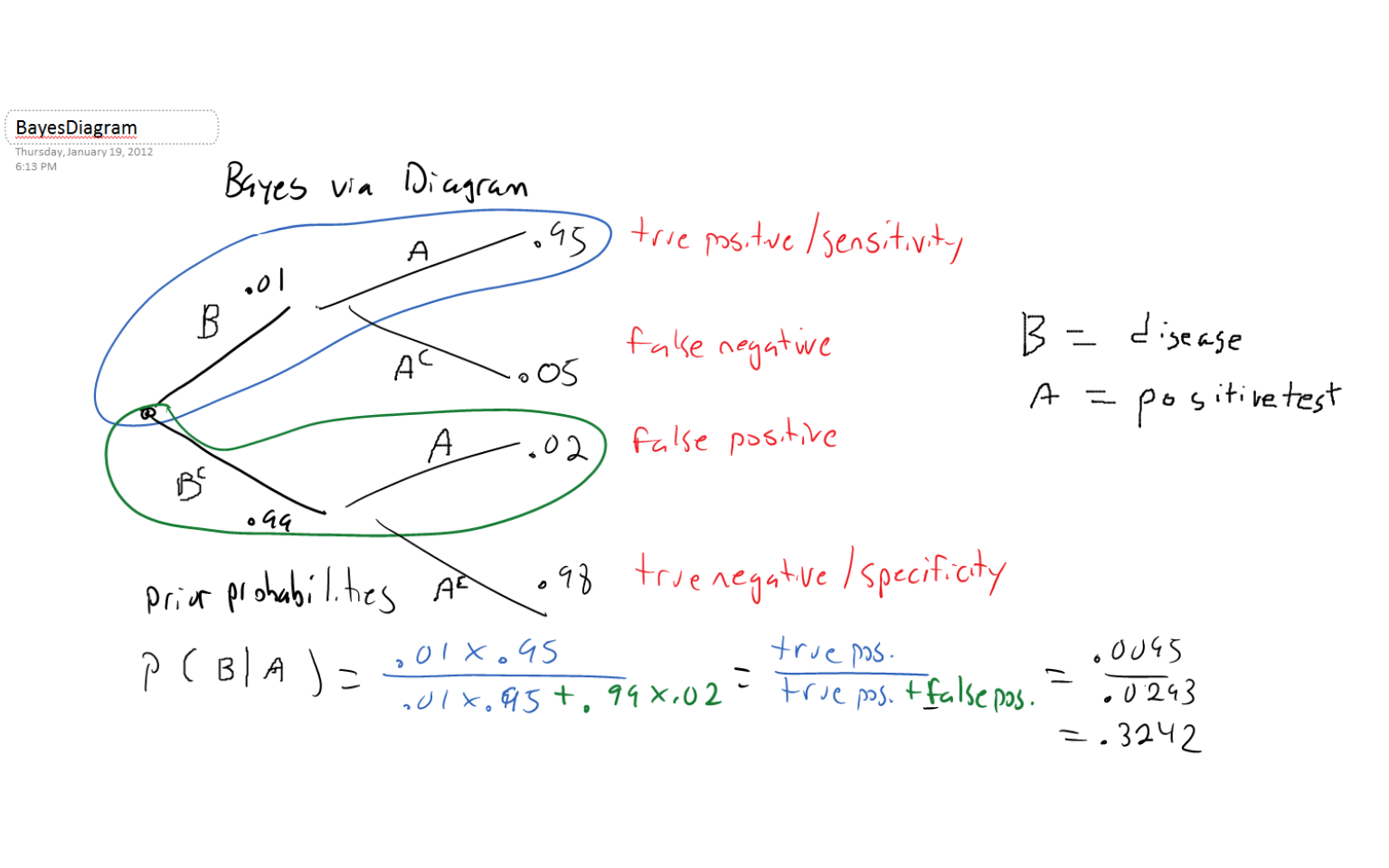
Notice that $P(D^+|T^+)$, the probability of having Martian flu if you had a positive test, is only 32.42%. This probability is so low because there are actually more ‘false positives’ than ‘true positives’ in the population.

This is often the case for rare diseases (i.e. low prevalence) unless sensitivity and specificity are incredibly close to 1.

While this will be the extend of our foray into Bayesian statistics, there is a large body of work in applied statistics that build upon the old reverend’s theorem for reversing probabilities!

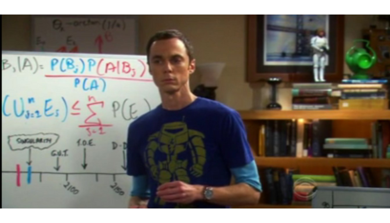
Sheldon Cooper from the sitcom The Big Bang Theory is using Bayes’ Theorem (with slightly different notation), along with a result called Boole’s Inequality. Boole’s Inequality is also known as the union bound and basically says that the probability of a union of events is no more than the sum of the individual probability of each event in the union.

\[P(\bigcup_{i=1}^{\infty}A_i) \leq \sum_{i=1}^\infty P(A_i)\]

I saw more Bayesian statistics on Sheldon’s whiteboard on a more recent episode, but I didn’t track down the screenshot.

1.6 Let’s Make a Deal

This is a pretty well-known problem, based on the game show Let’s Make a Deal. It is sometimes called the Monte Hall problem, after the host of the show back in the 1960s and 1970s.
There are three doors; behind one is a prize (say a car or lots of money which you want), and behind the other two is no prize (or something you don’t want). You choose a door, and the game show host shows you one of the doors you didn’t choose, where there is no prize. The host (Monte Hall or Wayne Brady) offers you a chance to switch to the other unopened door.
1. Should you switch doors?
2. Should you stay with your first choice?
3. Maybe it doesn’t matter and you could just flip a coin…
If you saw the TV show ‘Numb3rs’ or the movie ‘Twenty-One’, the problem was featured: http://youtu.be/OBpEFqjkPO8
You can simulate the game here: https://www.statcrunch.com/applets/type1&deal
Why is it better for you to switch your choice than stay with your initial guess? (You might draw a tree diagram to see why)

1.7 Simpson’s Paradox and Rates

As defined by the Stanford Encyclopedia of Philosophy, Simpson’s Paradox is a statistical phenomenon where an association between two variables in a population emerges, disappears or reverses when the population is divided into subpopulations. (Thanks to Dr. Randy Pruim for the reference, as discussed on an email list of statistics educators)

https://plato.stanford.edu/entries/paradox-simpson/

There are several famous examples of this paradox. Here, I’ll discuss a trivial example involving the batting averages of two professional baseball players, an example comparing the on-time rates of two airlines, along with a recent example (which might or might not be the paradox, but is useful in looking at the concept of rate and of conditional probability) involving the efficacy of vaccines against severe cases of COVID in Israel.

Other well-known examples that I won’t discuss here include: (1) possible gender discrimination in acceptance to graduate school at the University of California-Berkeley; (2) racial differences in the imposition of the death penalty in Florida; and (3) the effectiveness of different treatments for kidney stones

There’s a good Wikipedia page on Simpson’s paradox. The Wikipedia page has several other links, including some videos and a vector interpretation.

https://en.wikipedia.org/wiki/Simpson%27s_paradox

Baseball example

Derek Jeter and David Justice are both former professional baseball players that played for the New York Yankees and Atlanta Braves, respectively, during the 1995 and 1996 baseball seasons. As seen below, Jeter had a higher batting average (the proportion of base hits divided by at-bats, rounded by convention to three decimal places) than Justice when the two seasons are combined, but Justice had a higher batting average than Jeter for both the 1995 season and 1996 season when they are considered separately.

Year	Jeter	Justice
1995	12/48 = .250	104/411 = .253
1996	183/582 = .314	45/140 = .321
Both	195/630 = .310	149/551 = .270

You should notice that the sample sizes for the years are quite different: Jeter had the vast majority of his total at-bats in 1996 (he was first called up from the minor leagues at the end of the 1995 season) while Justice had the majority of his at-bats in 1995 (he missed much of the 1996 season due to injury).

Think about whether you would feel it is more important to judge the seasons separately or combined if you were trying to make a conclusion about which of these two players was a better hitter.

Note: a mathematician named Ken Ross has approximated that there should be about one such pair per year observed among major league players (I haven’t seen how he computed this).

Airline Example Alaska Airlines is an airline that has a “hub” in Seattle, while America West Airlines uses Phoenix as their “hub”. Let’s look at some data for the on-time performance of these airlines for five cities in the Western United States. (data from June 1991)

City	Alaska Airlines	America West
Los Angeles	497/559 = 88.9%	694/811 = 85.6%
Phoenix	221/233 = 94.8%	4840/5255 = 92.1%
San Diego	212/232 = 91.4%	383/448 = 85.5%
San Francisco	503/605 = 83.1%	320/449 = 71.3%
Seattle	1841/2146 = 85.8%	201/262 = 76.7%
Combined	3274/3775 = 86.7%	6438/7225 = 89.1%

Why does Alaska Airlines outperform America West in each city, but America West’s on-time percentage is higher overall?

If you could choose one of the two airlines, assuming that being on-time was of paramount importance to you and other factors (price, comfort, customer service, etc.) were the same, which would you choose?

Israel COVID infection example

Source: a post by Jeffrey Morris on August 17, 2021 to the Covid-19 Data Science blog, along with discussion of this article on an email list of statistics educators that I am a part of.

https://www.covid-datascience.com/post/israeli-data-how-can-efficacy-vs-severe-disease-be-strong-when-60-of-hospitalized-are-vaccinated

The nation of Israel has one of the highest rates of vaccination for COVID-19 in the world, with about 80% of the population aged 12 or older being fully vaccinated. However, on August 15, 2021, about 60% of the patients hospitalized for COVID in Israel were fully vaccinated. Should this cast doubt on the efficacy of being vaccinated?

On that date (8/15/2021), $n=515$ people were hospitalized in Israel with what was classified as a “severe” case of COVID.

$\:$	Population	%	Severe	Cases	Efficacy
Age	not vax	fully vax	not vax	fully vax	vs. severe cases
all			214	301	“does vaccination work???”

In this simple table, $301/515=0.584$, or 58.4% of the cases were in fully vaccinated Israelis vs. unvaccinated (this is ignoring a small percentage of the population that is currently partially vaccinated).

It was noted that there are important age-based differences in the vaccination rate. In Israel, about 90% of those aged 50 and over are fully vaccinated. About 85% of the unvaccinated population are under the age of 50.

There is also important age-based differences on the odds of having a severe case of COVID. In Israel, older people (50 and over) are about 20 times more likely to have a severe case than younger people (under 50). If we stratify age further and look at the extremes, Israelis aged 90 and over are about 1600 times more likely to have a severe case than Israelis aged 12-15 (the youngest people that can currently be vaccinated).

Below, we’ll look at adjusting for the vaccination rate. Again, a small portion of the Israeli population (about 3.1%) were partially vaccinated when this data was collected and are not included in the table below or used for the comparison between unvaccinated and fully vaccinated.

$\:$	Population	Values	Severe	Cases	Efficacy
Age	not vax	fully vax	not vax	fully vax	vs. severe cases
all	1,320,912	5,634,634	214	301	67.5%
$\:$	18.2%	78.7%	16.4 per 100K	5.3 per 100K

Severe cases were normalized by turning the raw number of cases (214 and 301, respectively) into a rate per 100,000 people. For example, in the unvaccinated: \[\frac{214}{1,320,912} \times 100,000 = 16.4\]

Dividing the rates per 100K people, we see \[\frac{16.4}{5.3}=3.1\] or a rate of severe cases that is about tripled among the unvaccinated vs. fully vaccinated.

A numerical measure of the efficacy of the vaccine is: \[1-\frac{V}{N}=1-\frac{5.3}{16.4}=0.675\]

When we say the efficacy of the vaccine is about 67.5%, this is saying that the vaccine is preventing over two-thirds of severe cases. This is lower than the 95% efficacy that had been the case with earlier variants of COVID, as the Delta variant is more serious.

Let’s see what happens if we stratify by age. The table below will report the population vaccinated/unvaccinated in each group as percentages, and the severe cases as rate per 100K people in that group. Efficacy is $100 \times (1-\frac{V}{N})$.

$\:$	Population	Values	Severe	Cases	Efficacy
Age	not vax	fully vax	not vax	fully vax	vs. severe cases
all	18.2%	78.7%	16.4	5.3	67.5%
$<50$	23.3%	73.0%	3.9	0.3	91.8%
$\geq 50$	7.9%	90.4%	91.9	13.6	85.2%

Notice that while the efficacy of the vacciine was 67.5% for the entire Israeli population, that this efficacy actually increased in both the under 50 group (to 91.8%) and the over 50 group (to 85.2%). Some consider this to be a case of Simpson’s Paradox (although some in the statistics educators group argued that this does not technically meet the definition, as the rate of severe cases is always higher among the unvaccinated). There’s a change in magnitude but not direction here.

I’m a fully vaccinated member of the $\geq 50$ group, where in Israel the rate per 100K of severe cases is 13.6, which is greater than the rate per 100K for non-vaccinated people under 50, which was 3.9. In Israel and many other nations, both vaccination status and the rate of severe COVID are systematically higher in the older age group, which is why it is important to stratify.

I won’t reproduce it here, but the article had a table with age stratified into 10 categories. Among those under 30, the vaccine efficacy was essentially 100%. Here, comparing fully vaccinated people in the 50-59 group versus non-vaccinated in the 20-29 age group in terms of rate per 100K is 2.9 to 1.5.

https://www.covid-datascience.com/post/israeli-data-how-can-efficacy-vs-severe-disease-be-strong-when-60-of-hospitalized-are-vaccinated

Matthew Brennaman found a case with data from the United Kingdom where there is Simpson’s Paradox. His data is drawn from Public Health England’s Technical Report 20, dealing with all cases of COVID that were identified as the Delta variant. In this data, fully and partially vaccinated are combined, and age data for some patients that did not die was unavailable.

https://assets.publishing.service.gov.uk/government/uploads/system/uploads/attachment_data/file/1009243/Technical_Briefing_20.pdf

Age	Delta Variant	COVID Cases	Number of	Deaths	Risk Ratio
$\:$	not vax	vax	not vax	vax	$\:$
all	151,054	117,115	253 (0.17%)	481 (0.41%)	0.41/0.17=2.4

Notice that the mortality rate (percentage of deaths) was higher in the vaccinated group. The risk ratio of vaccinated mortality rate to not vaccinated mortality rate is $0.41/0.17=2.4$.

But if we stratify by age (again, crudely as under 50 vs. 50 and older), the magnitude and direction of the relationship change. The risk ratios less than 1 indicate lower mortality rates among the vaccinated than the unvaccinated.

Age	Delta Variant	COVID Cases	Number of	Deaths	Risk Ratio
$\:$	not vax	vax	not vax	vax	vax to not vax
all	151,054	117,115	253 (0.17%)	481 (0.41%)	0.41/0.17=2.4
$<50$	147,612	89,807	48 (0.03%)	21 (0.02%)	0.02/0.03=0.7
$\geq 50$	3,440	27,307	205 (5.96%)	460 (1.68%)	1.68/5.96=0.3

Notice that the UK has lower vaccination ratesthan Israel, particularly among younger people.

STA 440/441 Notes (Mathematical Statistics I)