Chapter 3 Continuous Distributions
3.1 Random Variables of the Continuous Type
Suppose we have a continuous random variable \(X\) with support space \(S\), where \(S\) is either an interval or a union of intervals. It is common for the support space to be either all real numbers \(\mathbb{R}\) or all positive real numbers \(\mathbb{R}^+\). Sometimes the support will be an interval such as \([0,1]\) or more generally \([a,b]\), and in theory we could have the union of several such intervals.
The probability density function, or pdf, is an integrable function \(f: \mathbb{R} \to \mathbb{R}\) such that:
- \(f(x)\geq 0\) for all \(x \in \mathbb{R}\) (i.e. the pdf is never negative and is non-zero for values of \(x\) that are in \(S\))
- \(\int_{-\infty}^{\infty} f(x) dx=1\), and more specifically, \(\int_S f(x)dx=1\). (i.e. the area under the curve and above the \(x\)-axis is equal to 1 for a pdf)
- \(P(a \leq X \leq B)=P(a < X < b)=\int_a^b f(x) dx\) for all \(a \leq b\).
Recall that when when we dealt with inequalities for a discrete random variable \(X\), that \(P(X < a) \neq P(X \leq a)\). For example, if \(X \sim POI(\lambda=2.5)\), then \(P(X < 1)=P(X=0)\), but \(P(X \leq 1)=P(X=0)+P(X=1)\).
## [1] 0.082085## [1] 0.2872975## [1] 0.2872975However, for a continuous random variable, cumulative probabilities are not based on the sum of a discrete number of probabilities, but on area underneath the curve, i.e. \[Area \qquad \Longleftrightarrow \qquad Probability\]
For a continuous random variable \(X\) and any real number \(a\), the following are true:
\(P(X =a )=0\) because \[\int_a^a f(x) dx =0\]
\(P(X \leq a)=P(X < a)\) because \[P(X \leq a)=P(X < a) + P(X=a)=P(X < a)+0=P(X < a)\]
Similarly, \(P(X \geq a)=P(X > a)\)
The mean or expected value of a continuous random variable \(X\) is: \[\mu_X=E(X)=\int_S x f(x) dx\]
The variance of a continuous random variable \(X\) is: \[\sigma^2_X=Var(X)=\int_S (x-\mu_X)^2 f(x) dx\]
As this integral might be messy to evaluate, let’s simplify to a form that is generally easier to compute. I will let \(\mu=\mu_X\).
\[ \begin{aligned} Var(X) & = \int_S (x-\mu)^2 f(x) dx \\ & = \int_S (x^2-2\mu x + \mu^2) f(x) dx \\ & = \int_S x^2 f(x) dx -\int_S 2 \mu x f(x) dx + \int_S \mu^2 f(x) dx \\ & = \int_S x^2 f(x) dx - 2\mu \int_S x f(x) dx + \mu^2 \int_S f(x) dx \\ & = \int_S x^2 f(x) dx - 2\mu(\mu) + \mu^2(1) \\ & = \int_S x^2 f(x) dx - \mu^2 \\ & = E(X^2)-[E(X)]^2 \\ \end{aligned} \] ——————————————–
Continuous Uniform
Much as we did with discrete distributions, certain probability models occur frequently and we give specific names to these useful continuous probability distributions. The first we will consider is the continuous uniform distribution (usually just called the ‘uniform’).
A continuous random variable \(X\) is said to be uniform if all values of \(x\) over a given interval \([a,b]\), where \(a < b\), are equally likely and we say \(X \sim UNIF(a,b)\), where \[f(x)=\frac{1}{b-a}, x \in [a,b]\] and zero otherwise. It is quite common when computing pseduo-random numbers to base them on \(X \sim UNIF(0,1)\) (for instance, the rand function on a TI calculator generates such a value).
Graphically, this random variable’s pdf is represented by a rectangle of height \(\frac{1}{b-a}\) and width \(b-a\). Cumulative probabilites are computed by finding areas of rectangles!
Suppose \(X \sim UNIF(2,7)\)
## [1] 0.2## [1] 0#graph it
x<-seq(0,10,by=0.001)
f.x<-dunif(x=x,min=2,max=7)
plot(f.x~x,type="l")
#cdf function
#Find P(X<=3.4)
punif(q=3.4,min=2,max=7)## [1] 0.28#graph that region
tt<-seq(from=0,to=3.4,length=1001)
dtt<-dunif(tt,min=2,max=7)
polygon(x=c(2,tt,3.4),y=c(0,dtt,0),col="gray")
What is the expected value and variance of this distribution? Well, we could use R and definitions to compute them.
xf.x<-function(x) {x* 1/5 * (2<=x & x<=7)}
(E.x<-integrate(xf.x,2,7)$value) #E(X) is integral of x f(x)
## [1] 4.5## [1] 2.083333##
## Attaching package: 'MASS'## The following object is masked from 'package:dplyr':
##
## select## [1] 25/12It is not hard to derive for a uniform random variable \(X \sim UNIF(a,b)\) that \[E(X)=\frac{a+b}{2}\] \[Var(X)=\frac{(b-a)^2}{12}\]
With \(a=2\) and \(b=7\), we get \(E(X)=\frac{2+7}{2}=\frac{9}{2}\) and \(Var(X)=\frac{(7-2)^2}{12}=\frac{25}{12}\).
The triangular distribution
A continuous distribution \(X \sim f(x)\) is said to be triangular, if for constants \(a\) (the lower limit), \(b\) (the upper limit), and \(c\) (the mode of the triangle),
\[ \begin{aligned} f(x) = & 0 & x<a \\ = & \frac{2(x-a)}{(b-a)(c-a)} & a \leq x < c \\ = & \frac{2}{b-a} & x = c \\ = & \frac{2(b-x)}{(b-a)(b-c)} & c < x \leq b \\ = & 0 & x>b \\ \end{aligned} \]
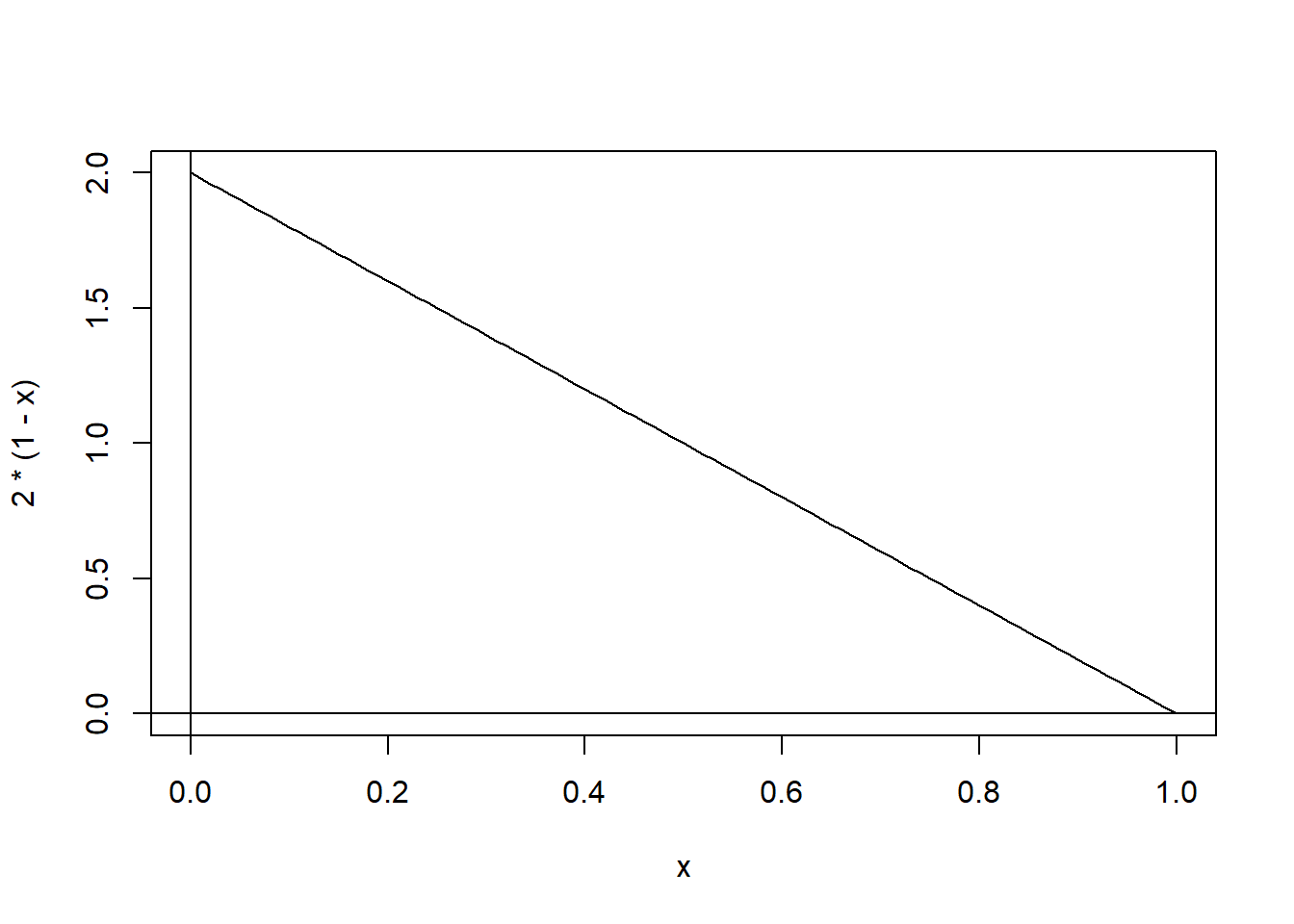
If we choose \(a=c=0\) and \(b=1\), then the pdf of \(X\) is \(f(x)=2(1-x), 0 \leq x \leq 1\), and zero otherwise. Our support space \(S_X=\{x: x \in [0,1]\}\).
(Draw the graph, it looks like a right triangle)
Is this a valid pdf?
Is the value of \(f(x)\) non-negative for all real numbers? Yes, \(f(x) \geq 0\) for all \(x \in \mathbb{R}\) and \(f(x)>0\) when \(x \in (0,1)\)
Is the area under the curve and above the \(x-axis\) equal to one? Yes, this can be verified both with simple geometry (i.e. find the area of the right triangle) or with calculus. \[\int_S f(x) dx = \int_0^1 2(1-x) dx = (2x-x^2)|_0^1 = 1 \]
We can find probabilities of being between specific values, such as \(P(\frac{1}{4} < X < \frac{3}{4})\)
curve(2*(1-x),from=0, to=1)
abline(a=2,b=-2) #y=a+bx
abline(v=0)
abline(h=0)
tt<-seq(from=0.25,to=0.75,length=100)
dtt<-2*(1-tt)
polygon(x=c(0.25,tt,0.75),y=c(0,dtt,0),col="gray")
\[ \begin{aligned} P(\frac{1}{4} < X < \frac{3}{4}) = & \int_{\frac{1}{4}}^{\frac{3}{4}} 2(1-x) dx \\ & = (2x-x^2)|_{\frac{1}{4}}^{\frac{3}{4}} \\ & = (\frac{6}{4}-\frac{9}{16})-(\frac{2}{4}-\frac{1}{16}) \\ & = \frac{1}{2} \\ \end{aligned} \]
It isn’t necessary here, or on most basic problems we will consider, but one could numerically approximate this integral using a TI calculator or R. Notice that the function command in R, used to define the pdf, essentially is using an Iverson bracket in its definition. We could say \[f(x)=2(1-x)[[0 \leq x \leq 1]], x \in \mathbb{R}\]
fun<-function(x) {2*(1-x) * (0 <= x & x <=1)}
integrate(fun,0,1) #verify probability under entire pdf is 1
## 1 with absolute error < 1.1e-14## 0.4375 with absolute error < 4.9e-15## 0.0625 with absolute error < 6.9e-16## 0.5 with absolute error < 5.6e-15## [1] 1/16Just by looking at the graph (and easily verified with simple calculus), we see that \(P(X \leq \frac{1}{4}) > P(X \geq \frac{3}{4} )\) and it seems reasonable that the expected value would be less than \(\frac{1}{2}\).
\[ \begin{aligned} E(X) & = \int_0^1 x f(x) dx \\ = & \int_0^1 x \cdot 2(1-x) dx \\ = & \int_0^1 2x-2x^2 dx \\ = & (x^2-\frac{2}{3}x^3)|_0^1 \\ = & \frac{1}{3} \\ E(X^2) & = \int_0^1 x f(x) dx \\ = & \int_0^1 x^2 \cdot 2(1-x) dx \\ = & \int_0^1 2x^2-2x^3 dx \\ = & (\frac{2}{3}x^3-\frac{1}{2}x^4)|_0^1 \\ = & \frac{1}{6} \\ Var(X) & = E(X^2)-[E(X)]^2 \\ & = \frac{1}{6}-(\frac{1}{3})^2 \\ & = \frac{1}{18} \end{aligned} \] Recall for a discrete random variable, we defined \(F(x)=P(X \leq x)\) to be the cumulative distribution function or cdf, of \(X\) and we founnd this very useful for computing probabilities. We have a very similar definition for continuous random variables; of course, we will integrate rather than taking a summation.
\[F(x)=P(X \leq x)=\int_{-\infty}^x f(t) dt\]
In many situations, we can derive formulas for the cdf of a continuous random variable. Suppose we have a friend that knows no calculus and cannot evaluate even the simplest of integrals and wouldn’t be able to use technology to numerically approximate integrals either. However, if we give them a formula to “plug” \(x\) into, they can probably do it.
Let’s derive the cdf for our earlier example.
\[F(x)=P(X \leq x)=\int_0^x 2(1-t)=(2t-t^2)|_0^x=2x-x^2\]
Hence, our cdf is: \[ \begin{aligned} F(x) & = 0 & x < 0 \\ & = 2x-x^2 & x \in [0,1] \\ & = 1 & x > 1 \\ \end{aligned} \]
So, \[P(X \leq \frac{1}{4})=F(\frac{1}{4})=2(\frac{1}{4})-(\frac{1}{4})^2=\frac{7}{16}=0.4375\] \[P(X \geq \frac{3}{4})=1-F(\frac{3}{4})=1-[2(\frac{3}{4})-(\frac{3}{4})^2]=1-\frac{15}{16}=\frac{1}{16}=0.0625\]
Suppose I want the median of my distribution. Graphically, the median would be the point such that exactly half of the area under the curve is less than the median, and the other half is greater than the median.
curve(2*(1-x),from=0, to=1)
abline(a=2,b=-2) #y=a+bx
abline(v=0)
abline(h=0)
tt<-seq(from=0,to=(2-sqrt(2))/2,length=100)
dtt<-2*(1-tt)
polygon(x=c(0,tt,(2-sqrt(2))/2),y=c(0,dtt,0),col="gray")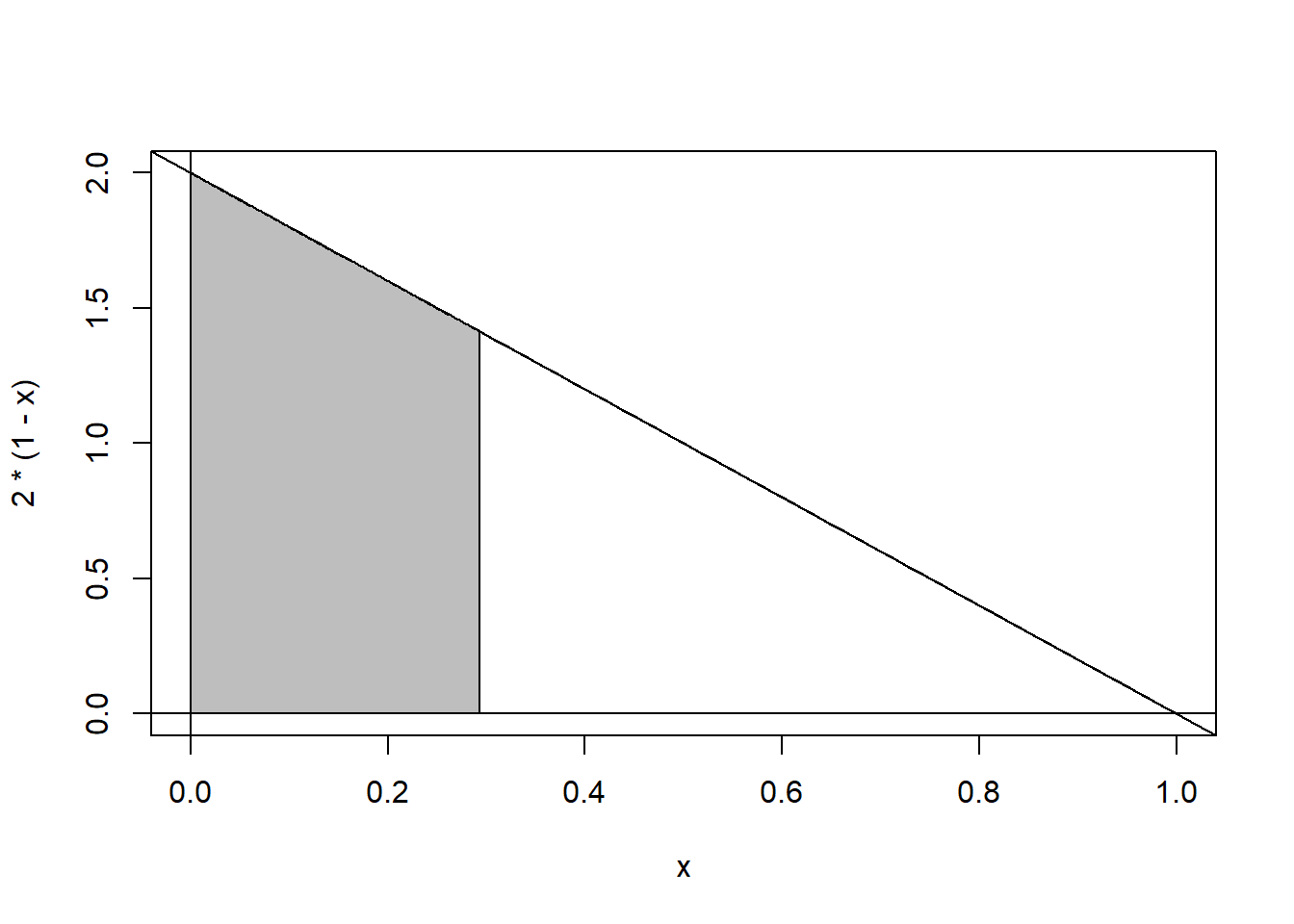
If we let \(m\) represent the median, then clearly \(F(m)=P(X \leq m)=0.50\).
\[ \begin{aligned} F(m) & = 0.5 \\ 2m-m^2 & = 0.5 \\ 0 & = m^2-2m+0.5 \\ \end{aligned} \]
Using the quadratic formula, we find that \[m=\frac{-(-2) \pm \sqrt{(-2)^2-4(1)(0.5)}}{2(1)}=\frac{2 \pm \sqrt{2}}{2} \approx 1.707,0.293\]
Since \(\frac{2+\sqrt{2}}{2}\) is greater than 1, it cannot be the median, hence \[m=\frac{2-\sqrt{2}}{2}\]
We can find other quantiles \(q\) by using values other than 0.5. For example, if you solved \(q^2-2q+0.25=0\) for \(q\), you would find the 25th percentile or first quartile of the distribution.
3.2 The Exponential, Gamma, and Chi-Square Distributions
The Gamma Distribution
Before we can study the pdf of the gamma distribution, we need to introduce the so-called gamma function.
Definition: The gamma function is defined for \(\alpha>0\) as \[\Gamma(\alpha)=\int_0^{\infty} y^{\alpha-1} e^{-y} dy\]
Notice that if \(\alpha=1\), then \[\Gamma(1)=\int_0^{\infty} e^{-y} dy-1\]
If \(\alpha\) is an integer greater than one, we can obtain a recursive formula to evaluate the gamma function. \[\Gamma(\alpha)=\int_0^{\infty} y^{\alpha-1} e^{-y} dy\]
Use integration by parts with \(u=y^{\alpha-1}\) and \(dv=e^{-y} dy\), so \(du=(\alpha-1)y^{\alpha-2}\) and \(v=-e^{-y}\).
So \[ \begin{aligned} \Gamma(\alpha) & =\lim_{L \to \infty} y^{\alpha-1}(-e^{-y})|_0^L + \int_0^{\infty} (\alpha-1)y^{\alpha-2}e^{-y} dy \\ & = 0 + (\alpha-1) \int_0^{\infty} y^{(\alpha-1)-1}e^{-y}dy \\ & = (\alpha-1)\Gamma(\alpha-1) \\ \end{aligned} \]
Using mathematical induction, we eventually obtain that \(\Gamma(\alpha)=(\alpha-1)!\) for any positive integer \(\alpha\). For example, \(\Gamma(5)=4\Gamma(4)=4\times 3\Gamma(3)=4\times 3 \times 2\Gamma(2)=4 \times 3 \times 2 \times 1\Gamma(1)=4 \times 3 \times 2 \times 1\).
Now we give the pdf of the gamma distribution with shape paramter \(\alpha\) and scale parameter \(\theta\). Note: Many books use different notation and some use a different parametrization than our book, defining \(\lambda=1/\theta\) as a rate parameter.
\[f(x;\alpha,\theta)=\frac{1}{\Gamma(\alpha) \theta^\alpha} x^{\alpha-1} e^{-x/\theta}\] where \(x,\alpha,\theta>0\).
We say \(X \sim GAMMA (\alpha, \theta)\). When \(\alpha=1\), the distribution reduces to an exponential distribution \(X \sim EXP(\theta)\) where \[f(x)=\frac{1}{\theta}e^{-x/\theta}, \: x,\theta>0\]
The mean, variance, and moment-generating function are given below:
\[E(X)=\alpha\theta, Var(X)=\alpha \theta^2, M_X(t)=(\frac{1}{1-\theta t})^{\alpha}, t< \frac{1}{\theta}\]
No functions for this distribution are given on the TI-84, but the usual suite of d-, p-, q-, and r-operators are available in R. In the code below, I will graph \(X \sim GAMMA(\alpha=3,\lambda=0.5)\), find \(F(5)=P(X<5)\), and find the 60th percentile of the distribution. Note that \(E(X)=6\) and \(Var(X)=12\). Note that in R that the \(\alpha\) parameter is specified with shape and the \(\theta\) parameter with scale. If you use the parameterization with \(\lambda = \frac{1}{\theta}\), you would use rate to specify the value of \(\lambda\).
x<-seq(0,15,by=0.001)
f.x<-dgamma(x=x,shape=3,scale=2) #alpha=3, theta=2
plot(f.x~x,type="l",main="Gamma pdf with alpha=3, theta=2")
tt<-seq(from=0,to=5,length=1000)
dtt<-dgamma(x=tt,shape=3,scale=2)
polygon(x=c(0,tt,5),y=c(0,dtt,0),col="gray")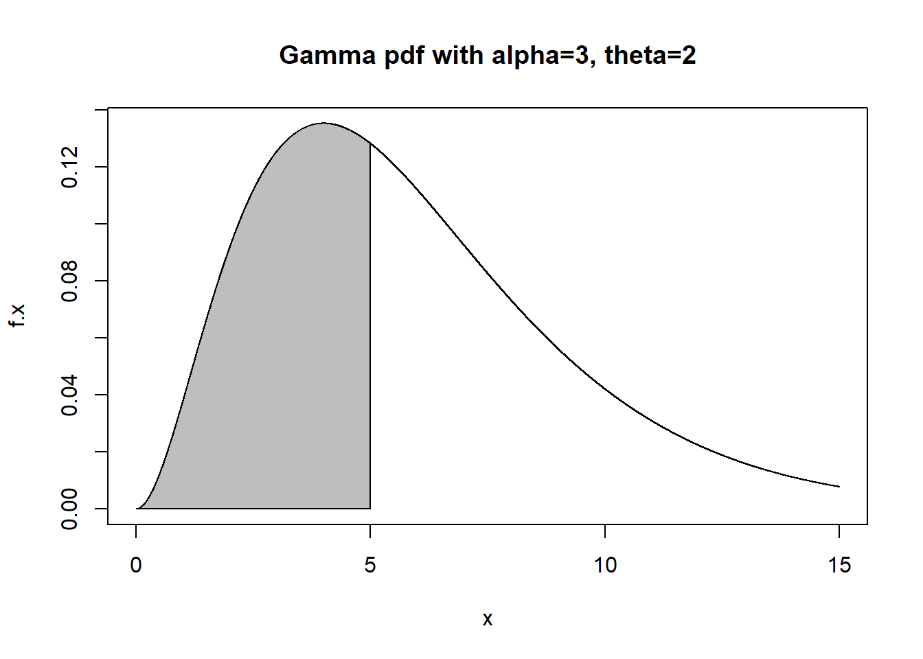
## [1] 0.4561869## [1] 0.4561869## [1] 6.210757The special case of the gamma distribution where \(\alpha=1\) is called the exponential distribution, with parameter \(\theta=\frac{1}{\lambda}\).
\[f(x)=\frac{1}{\theta}e^{-x/\theta}, \: 0 \leq x < \infty, \theta>0\] \[f(x)=\lambda e^{-\lambda x}, \: 0 \leq x < \infty, \lambda=0\]
We denote this as \(X \sim EXP(\theta)\) Note that the expected value and variance of the exponential are: \[E(X)=\theta\] \[Var(X)=\theta^2\]
The cdf is easily found:
\[ \begin{aligned} F(x) & = \int_0^x \lambda e^{-\lambda t} dt \\ & = \lambda \cdot -\frac{1}{\lambda} e^{-\lambda t}|_0^x \\ & = -e^{\lambda t}|_0^x \\ & = -e^{\lambda x}--e^0 \\ & = 1-e^{\lambda x} \\ \end{aligned} \]
We, of course, have functions in R to compute the pdf and cdf of the exponential distribution. R uses rate as the parameter, which is \(\lambda=1/\theta\).
Let’s do an example where \(X \sim EXP(\theta=2)\), where we want to find \(P(1 < X < 4)=F(4)-F(1)\).
## [1] 0.3032653## [1] 0.06766764## [1] 0.3934693## [1] 0.8646647## [1] 0.3495638Relationship between exponential and Poisson distributions
Suppose a discrete random variable \(X\) represents the number of flaws in a 1 meter length of fiber-optic cable and \(X\) is assumed to follow a Poisson process so that \(X \sim POI(\lambda)\); that is, on average we expect \(\lambda\) flaws per 10 meter length of cable. We might observe \(X=0\) or \(X=2\) or any non-negative integer value.
Now define a continuous random variable \(Y\) and have it represent the distance until the next flaw is found. We might observe \(Y=0.2\) or \(Y=1.52\) or \(Y=\pi+e\) or any non-negative real value.
The CDF of \(Y\) is \(F(y)=P(Y \leq y)=1-P(Y > y)\). If we realize that \(P(Y > y)\) represents the probability of zero occurrences (in our example, flaws in a length of cable) from \([0,y]\), then \(P(Y>y)\) is equivalent to \(P(W=0)\), where \(W\) represents the number of flaws in a \(y\) meter length of cable. Since \(X \sim POI(\lambda)\), then \(W \sim POI(y \lambda)\).
Hence \[F(y)=1-P(W=0)=1-\frac{e^{-\lambda y}(\lambda y)^0}{0!}=1-e^{-\lambda y}\]
If you don’t recognize that the CDF of \(Y\) is that of the exponential distribution, take the derivative.
\[f(y)=F'(y)=\lambda e^{-\lambda y}\]
which is the pdf of the exponential distribution.
This means that if we have a Poisson random variable \(X\), we can model the length of the interval (i.e. waiting time, length of wire, etc.) \(Y\) as an exponential random variable.
Example: Suppose the number of flaws per 10 meters of wire follows a Poisson distribution with \(\lambda=2.5\). Find the probability that no flaws are found in the next 5 meters of wire.
Solution (#1): I find this problem easier to consider letting \(X\) represent the Poisson process for 1 meter lengths. Since \(\lambda=2.5\) for a 10 meter interval, then \(\lambda=\frac{2.5}{10}=0.25\) for a 1 meter length and \(X \sim POI(\lambda=0.25)\).
Now, let \(Y\) represent the length of wire until the next flaw is found. We know that \(Y \sim EXP(\lambda=2.5)\). To find the probability that no flaws are found in the next 5 meters, we want \(P(Y > 5)\), or \(1-P(Y \leq 5)=F(5)\).
Using the CDF of the exponential, \(F(5)=1-(1-e^{-0.25(5)})=e^{-1.25}=0.2865\)
## [1] 0.2865048## [1] 0.2865048Solution (#2): Instead of rescaling \(X\) from a 10 meter to a 1 meter length of cable, you could instead rescale \(Y\). Let \(X \sim POI(\lambda=2.5)\) for 10 meter lengths of cable. Since 5 meters is half of 10 meters, find \(P(Y>0.5)\) when \(Y \sim EXP(\lambda=2.5)\).
\(F(0.5)=1-(1-e^{-2.5(0.5)})=e^{-1.25}=0.2865\)
## [1] 0.2865048Solution (#3): You can also solve by using the Poisson pdf rather than the exponential cdf. This time, we will need to scale \(\lambda\) in relation to 5 meter lengths of cable. If \(\lambda=0.25\) for 1 meter lengths, multiply by 5, or equivalently, if \(\lambda=2.5\) for 10 meter lengths, divide by 2. Either way, \(\lambda=1.25\). \(X\) will represent the number of flaws in 5 meters of wire, \(X \sim POI(\lambda=1.25)\). To find the probability that we go more than 5 meters before finding the first flaw, we find \(P(X=0)\).
\(f(0)=\frac{e^{-1.25}1.25^0}{0!}=e^{-1.25}=0.2865\)
## [1] 0.2865048The Relationship between Gamma & Poisson Distributions
Suppose we have a Poisson process (maybe we are observing the number of cars that pass a particular location). Let some random variable \(W\) represent the waiting time (or length of the interval) that is needed for exactly \(k\) events to occur. The cdf of \(W\) is \[G(w)=P(W \leq w)=1-P(W>w)\]
We realize that the event \(W>w\) (as long as \(w>0\)) is equivalent to the event where we observe less than \(k\) events in the interval \([0,w]\). So if \(X\) is the Poisson random variable that looks at the number of events in that interval \([0,w]\), then \(X \sim POI(\lambda w)\) where \(\lambda\) would be the rate in an interval of length 1.
So \[P(W > w)=P(X < k)=\sum_{x=0}^{k-1} \frac{e^{-\lambda w} (\lambda w)^x}{x!}\]
It can be shown (we’ll skip the details) through integration by parts a total of \(k-1\) times that
\[\int_\mu^\infty \frac{1}{\Gamma(k)}z^{k-1} e^{-z} dz = \sum_{x=0}^{k-1} \frac{\mu^x e^{-\mu}}{x!}, k=1,2,3,\cdots\]
Accepting that is true, then let \(\lambda w=\mu\) and we obtain \[G(w)=1-P(W > w)=1-\int_{\lambda w}^\infty \frac{1}{\Gamma(k)} z^{k-1} e^{-z} dz\]
for \(w>0\); of course, \(G(w)=0\) when \(w \leq 0\). Substitute \(z=\lambda y\) and hence \(dz=\lambda dy\) and \(y=\lambda/z\) into the above integral, we get:
\[G(w)=\int_0^w \frac{1}{\Gamma(k)} \lambda^k y^{k-1} e^{-\lambda y} dy\]
You should recognize the integral as being \(Y \sim GAMMA(\alpha=k,\lambda)\). We can then let \(\theta=\frac{1}{\lambda}\) to obtain our book’s parameterization, although I think that the \(\lambda\) as rate parameter is a good choice when showing the relationship between the gamma and Poisson distributions.
Example: Assume (unrealistically) that cars drive down a remote country road at a rate of \(\lambda=3\) cars per hour. What is the probability that we would wait over 45 minutes before observing the second car?-
Solution #1: Let \(X \sim POI(\lambda=3)\) represent the count of cars per hour. I will convert minutes to hours, so we are looking for the probability that we wait more than 0.75 hours before observing the second car. This waiting time will follow a gamma distribution, \(W \sim GAMMA(\alpha=2,\lambda=3)\).
We want \(P(W>0.75)=1-F(0.75)\). You could integrate by parts to solve
\[1-\int_0^{0.75} \frac{1}{\Gamma(2)} 3^2 w^{2-1} e^{-3w} dw=1-\int_0^{0.75} 9w e^{-3w} dw\] by choosing \(u=9w\) and \(dv=e^{-3w}dw\) so that \(du=9 dw\) and \(v=-\frac{1}{3}e^{-3w}\). You end up getting \(\frac{13}{4}e^{-9/4}\).
or use R.
## [1] 0.3425475## [1] 0.3425475Solution #2: If you prefer minutes rather than hours as your unit of measurement, then \(X \sim POI(\lambda=\frac{3}{60}=\frac{1}{20})\) and \(W \sim GAMMA(\alpha=2,\lambda=\frac{1}{20})\). We want \(P(W>45)=1-F(45)\).
## [1] 0.3425475Solution #3: We can solve by summing the Poisson pmf rather than integrating the gamma pdf. If cars arrive at a rate of \(\lambda=3\) per hour, then they would arrive at a rate \(\lambda=3 \times \frac{3}{4}=\frac{9}{4}\) per 45 minutes. Let \(Y \sim POI(\lambda=\frac{9}{4})\), so the probability of waiting longer than 45 minutes for the second car is equal to \(P(Y \leq 1)\), the probability of having observed either zero cars or one car in a 45 minute interval.
## [1] 0.3425475Chi-Squared Distribution (briefly)
A special case of the gamma distribution that will be important later is the chi-squared distribution. If we choose the gamma parameters such that \(\alpha=\frac{r}{2}\) and \(\theta=2\), then the resulting distribution is said to be chi-squared with \(r\) degrees of freedom, or \(X \sim \chi^2(r)\).
\[f(x)=\frac{1}{\Gamma(r/2)2^{r/2}}x^{r/2-1}e^{-x/2}, \: 0 < x < \infty\]
The mean and variance are \(\mu=r\) and \(\sigma^2=2r\), respectively.
Graphing and finding area under the curve for the chi-square distribution can be done with R, and there is a chi-square CDF function on TI calculators as well, where the only parameter you need is the degrees of freedom. For example, suppose \(X \sim \chi^2(df=3)\) and we wish to know \(P(X \leq 7.25)\) and the 95th percentile.
x<-seq(0,15,by=0.001)
f.x<-dchisq(x=x,df=3)
plot(f.x~x,type="l",main="Chi-square pdf with df=3")
tt<-seq(from=0,to=7.25,length=1000)
dtt<-dchisq(x=tt,df=3)
polygon(x=c(0,tt,7.25),y=c(0,dtt,0),col="gray")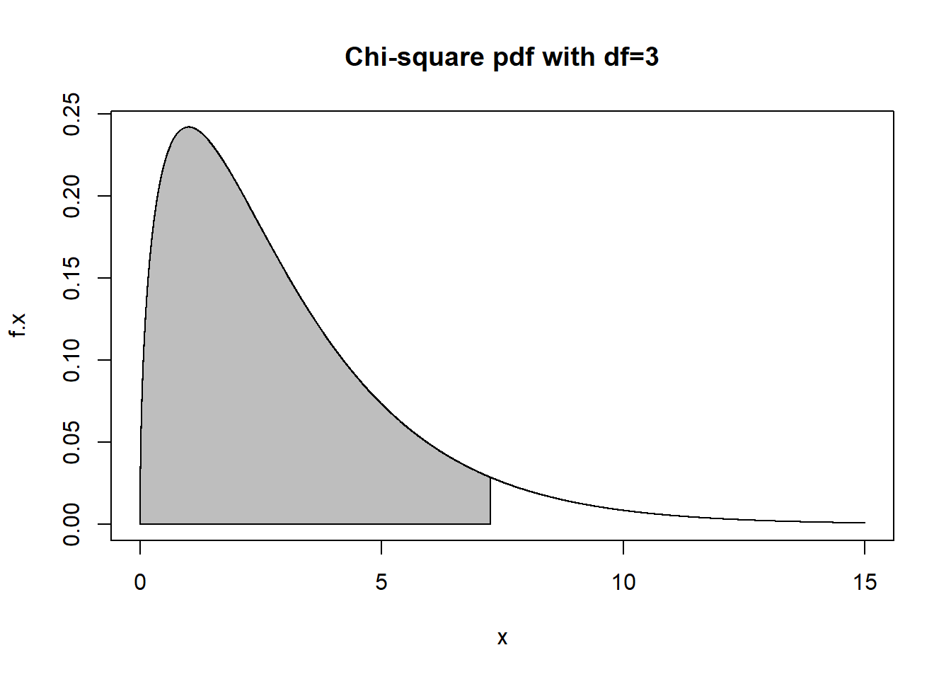
## [1] 0.9356578## [1] 0.9356578## [1] 9.487729We will see later that the chi-squared distribution is related to the normal distribution and is very useful in certain types of statistical testing. The so-called chi-squared tests that you may have heard of are based on hypothesis tests whose test statistics have distributions that are \(\chi^2\) under the null, and the distribution is also very important in likelihood ratio tests. We will delay further discussion of it until then.
3.3 The Normal Distribution
The normal distribution is a continuous probability distribution that is probably the single most important distribution in statistics. It is known to laymen as the ‘bell curve’ and is also sometimes called the Gaussian distribution after the German mathematician Karl Friedrich Gauss.
Normal curves have the following properties:
continuous
unimodal
‘bell’ shaped
symmetric (mean=median=mode)
asymptotic
the inflection points are located at exactly \(\mu \pm \sigma\)
Let’s look at the graph of \(X \sim N(100,15)\), which might describe scores obtained on a so-called ‘IQ’ test.

The normal distribution is important because it serves as a good model for many physical phenomenon that we study (such as the height or weight of a biological organism) and for measurement errors. Furthermore, it has many desirable theoretical properties that make sums or averages from non-normal populations have a sampling distribution that is approximately normal. We’ll study this in detail later, as the Central Limit Theorem.
A normal random variable \(X\) is described by two parameters, \(\mu\) and \(\sigma\), which serve as the mean and standard deviation of the population. We say \[X \sim N(\mu,\sigma)\] Many standardized tests are created in such a way as to yield distributions that are approximately normal with differing values for these parameters. For example, suppose I take both the SAT and ACT exams, and we’ll look at our score on the mathematics portions of those exams. Using \(X\) and \(Y\), respectively, for the SAT and ACT we have \[X \sim N(500,100)\] and \[Y \sim N(20,5)\]
These scales are quite different, and there is no theoretical basis for preferring the scale chosen by either of the testing companies. Suppose Pat took both exams, obtaining \(x=640\) and \(y=28\). Which test did Pat do better on? It’s not as simple as just saying Pat did better on the SAT because \(x>y\). If Pat had gotten \(x=400\), that would have been below average on the SAT, while \(y=28\) is above average on the ACT.
We deal with this problem by computing what are known as standardized scores or \(z\)-scores. The concept is to rescale both random variables onto a common scale, and the resulting \(z\)-score measures how many standard deviations above or below average an observation is. All we do is ‘center’ the value by subtracting the mean, and then divide by the standard deviation.
\[z=\frac{x-\mu}{\sigma}\]
If \(X \sim N(\mu,\sigma)\), then the resulting random variable \(Z\) is standard normal, with mean zero and standard deviation one. \[Z \sim N(0,1)\]
For Pat, the \(z\)-scores are: \[z_X=\frac{640-500}{100}=1.4, z_Y=\frac{28-20}{5}=1.6\]
While Pat was over one standard deviation above average on both exams, the \(z\)-score was a bit higher on the ACT, and thus Pat did better on the ACT exam than on the SAT exam.
I could report your exams scores in this class to you in terms of \(z\)-scores, but you might not like getting a negative score, which will happen if you are below average. For example, Dr. Mecklin’s \(z\)-score for height, using adult American men as our population, would be negative because I am shorter than the average adult American man. My sister is the same height as me, but her \(z\)-score for height would be positive because she is taller than the average adult American woman.
Usually, when you take a standardized exam such as the SAT or ACT, your score is reported to you both as a raw score \(X\) and as a percentile, and is almost never reported to you as a \(z\)-score. Why? Many people are not familiar with standardized scores and standard deviations, so knowing that their \(z\)-score on the SAT they got \(x=640\) on is \(z=1.40\) is not meaningful. But, knowing that a score of \(x=640\) is at the 92nd percentile is useful; this means this person scored higher than 92% of the population on the SAT. But how did I know it was 92%, instead of 52% or 82% or 99.2%?
Well, the normal distribution is a continuous probability distribution, so it will have a pdf and finding percentiles is just finding area underneath the curve, i.e. solving some integral.
The pdf of \(X \sim N(\mu,\sigma)\) is \[f(x)=\frac{1}{\sqrt{2\pi \sigma^2}} e^{-(x-\mu)^2/2\sigma^2}\] for \(-\infty \leq x \leq \infty\), \(-\infty \leq \mu \leq \infty\), \(\sigma>0\). That looks like it would be horrendous to try and evaluate; in fact, there is no analytic solution and when we evaluate a definite integral based on the normal, we have to use a numerical approximation that was either tabled or available on a calculator or computer.
Verifying that \(\int f(x) dx=1\) is somewhat laborious and involves a nifty change of variables to polar coordinates (refer to pages 105-106 for the fun details). The mgf for the normal distribution is \[M_X(t)=e^{\mu t + \sigma^2 t^2/2}\] which reduces to \(M_Z(t)=e^{t^2/2}\) for the standard normal.
The tables that were traditionally used were based on the standard normal distribution, i.e. \(Z \sim N(0,1)\) with pdf \[\phi(z)=\frac{1}{\sqrt{2 \pi}}e^{-z^2/2}\] Note that it is traditional to use a lower case phi (\(\phi\)) for the standard normal density function; similarly, we will use upper case phi, \(\Phi\), for the cdf. That is \(\Phi(1)=P(Z \leq 1)\).
Normal Distribution Calculations
The dnorm function in R or the corresponding normalpdf() function on a TI-calculator is used to evaluate the pdf \(f(x)\) or \(\phi(z)\) for a normal distribution. We rarely do this except when graphing.
## [1] 0.001497275#phi(1.4), use normalpdf(1.4) on TI-84
dnorm(x=1.4) #phi(1.4), notice not equal to previous calculation## [1] 0.1497275#graph it
x<-seq(200,800,by=0.001) #graphing from 3 sd below to 3 sd above the mean
f.x<-dnorm(x=x,mean=500,sd=100)
plot(f.x~x,main="X ~ N(500,100)",type="l")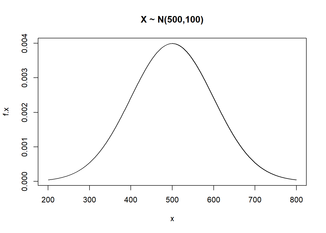

Usually, we want to find areas under the curve by evaluating the cdf \(F(x)\) or \(\Phi(z)\).
Suppose \(X \sim N(500,100)\) and I want to find the probability of getting a 640 or less on the exam, i.e. \(P(X \leq 640)=F(640)\).
#graph it
x<-seq(200,800,by=0.001) #graphing from 3 sd below to 3 sd above the mean
f.x<-dnorm(x=x,mean=500,sd=100)
plot(f.x~x,main="X ~ N(500,100), P(X<=640)",type="l")
tt<-seq(from=200,to=640,length=1000)
dtt<-dnorm(x=tt,mean=500,sd=100)
polygon(x=c(200,tt,640),y=c(0,dtt,0),col="gray")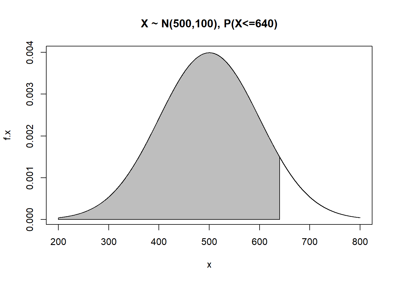
## [1] 0.9192433## [1] 0.9192433We see that \(P(X \leq 640)=F(640)\) or equivalently \(P(Z \leq 1.4)=\Phi(1.4)\) is 0.9192, or about 92%. This is why someone with a score of \(x=640\) on the mathematics SAT is at the 92nd percentile.
What if I know a percentile and want to work the problem backwards? For instance, suppose I need to be in the top 15% of students on the SAT to get accepted to Snooty U. You probably want to know what score is needed.

Obviously, the top 15% is equivalent to the 85th percentile or the \(0.85\)-quantile. One way of solving this problem is to find the \(z\)-score associated with the 85th percentile.
## [1] 1.036433The ‘needed’ \(z\)-score to be in the top 15% (the 85th percentile), is \(z=1.04\). Another way of saying this is that \(\Phi^{-1}(0.85)=1.04\). We are using the inverse of the CDF of the standard normal distribution. Plug into the \(z\)-score formula and solve for \(x\).
\[ \begin{aligned} z & =\frac{x-\mu}{\sigma} \\ 1.04 & = \frac{x-500}{100} \\ x & = 500 + 1.04(100) \\ x & = 604 \\ \end{aligned} \]
So the needed score is about \(X=604\). More directly:
## [1] 603.6433The rnorm function, or RandNorm on the TI-84, generates random normal variates.
##  [1] 625.8980 655.1127 425.2373 524.0998 453.3466 306.7286 555.2124 369.8057
##  [9] 356.3214 645.4199 564.6125 459.3300 395.5976 429.3729 419.6747 434.1611
## [17] 398.0744 369.1195 580.1093 485.90053.4 Additional Models
Memoryless property, Survival and Hazard Functions
Much like the geometric distribution was the only discrete distribution that is memoryless, the exponential distribution is the only continuous distribution with this property.
If \(X \sim EXP(\lambda)\), what is \(P(X>b|X>a)\), where \(0 < a < b\)? (The derivation is essentially the same if you use \(\theta=1/\lambda\) as the parameter).
\[ \begin{aligned} P(X > b | X > a) & = \frac{P(X >b)}{P(X > a)} \\ & = \frac{1-(1-e^{-\lambda b})}{1-(1-e^{-\lambda a})} \\ & = \frac{e^{-\lambda b}}{e^{-\lambda a}} \\ & = e^{-\lambda(b-a)} \\ & = P(X > b-a) \\ \end{aligned} \]
In other words, the probability only depends on the difference \(b-a\). For example, if \(X\) represented the waiting time until the 1st failure of a computer’s operating system, then the probability of ‘surviving’ (not failing) until time \(b\) does NOT depend on how ‘old’ the system is, where we can define the survival function as the complement of the cdf.
\[S(t)=1-F(t)=1-P(X < t)=P(X>t)\] For the exponential distribution, the survival function is \(S(t)=e^{-\lambda t}\).
For instance, if \(a=10000\) hours and \(b=25000\) hours, then the probability of surviving beyond 25000 hours, if the system has already run for 10000 hours, is equal to the probability that a new system survives for 25000-10000=15000 hours. The exponential distribution assumes the probability of a failure is the same at any point of time.
If this strikes you as unrealistic, you are correct in most real-life scenarios. Parts are more likely to fail as they wear out; humans or other biological organisms are more likely to die as they get older. More complicated distributions such as the Weibull distribution can model more realistic situations, where the probability of a failure is NOT constant but changes over time.
The hazard function gives the instantaneous probability of the event occurring at time \(t\), given that one has survived without the event occurring until time \(t\). It is the ratio of the density function and the survival function for a distribution. The hazard function for the exponential is:
\[H(t)=\frac{f(t)}{S(t)}=\frac{\lambda e^{-\lambda t}}{e^{-\lambda t}}=\lambda\]
The exponential distribution assumes a constant hazard!
Your book uses the notation \[\lambda(w) = \frac{g(w)}{1-G(w)}\], where \(W\) represents the survival time of an item and \(\lambda(w)\) is called the failure rate or force of mortality. This failure rate or force of mortality or hazard is unrealistically assumed to be constant with the exponential distribution, as an increasing function would be more realistic in most settings (i.e. a part wears out over time or a biological organism ages and is more likely to die when old). If this hazard were constant, then a 50 year old professor would be as likely to be alive 30 years from now as a 20 year old student, but this is not true.
The Weibull Distribution
Recall that the exponential distribution has the memoryless property, which renders it as being usually unrealistic to model survival, such as the waiting time until a part fails or a biological organism dies. A more complicated but realistic distribution, which does not have this property, is called the Weibull distribution. Different choices of the shape parameter \(\alpha\) and scale parameter \(\beta\) can model different scenarios such as ‘infant mortality’ or ‘old-age wearout’. \(X \sim WEI(\alpha,\beta)\). Notice that shape parameter \(\alpha=1\) will reduce to the exponential distribution.
\[f(x; \alpha, \beta)=\frac{\alpha}{\beta^{\alpha}} x^{\alpha-1} e^{-(x/\beta)^{\alpha}}\] for \(x, \alpha, \beta>0\). The expected value is \(E(X)=\beta \Gamma(1+\frac{1}{\alpha})\).
#Weibull program
#plot Weibull curves for ball bearing lifetime, in hours
#X~WEI(alpha=2,beta=40000), Y~WEI(alpha=1.3,beta=40000)
options(scipen=10)
(E.X<-40000*gamma(1+1/2))
## [1] 35449.08## [1] 36943.07bb<-seq(1,100000,by=1)
plot(dweibull(bb,shape=2,scale=40000)~bb,type="l",col="blue",xlab="Hours",ylab="Density")
points(dweibull(bb,shape=1.3,scale=40000)~bb,type="l",col="red")
points(dweibull(bb,shape=0.8,scale=40000)~bb,type="l",col="purple")
points(dnorm(bb,mean=35449.08,sd=18530.06)~bb,type="l",col="green")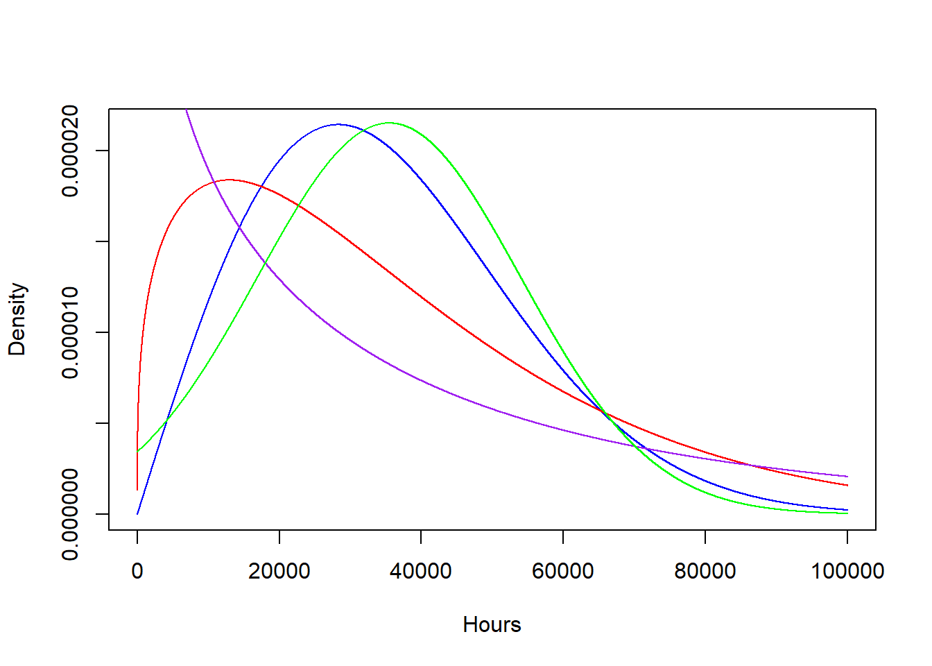
#the 3rd curve is a normal curve with same mean, sd as the 1st Weibull curve
#P(X>50000)
1-pweibull(q=50000,shape=2,scale=40000)
## [1] 0.2096114## [1] 0.2161505The Beta Distribution
The beta distribution is like the uniform distribution in that is is defined over a finite interval, in the case of the beta, \(x \in [0,1]\). We will see next semester that the beta distribution is extremely useful in modeling proportions. It has two shape parameters \(\alpha\) and \(\beta\), where the distribution is symmetric when \(\alpha=\beta\) and is equivalent to the \(UNIF(0,1)\) when \(\alpha=\beta=1\). When \(\alpha>\beta\), the distribution is left-skewed; when \(\alpha<\beta\) it is right-skewed. Larger values for \(\alpha\) and \(\beta\) lead to a smaller variance.
The pdf for \(X \sim BETA(\alpha,\beta)\) is: \[f(x)=\frac{\Gamma(\alpha+\beta)}{\Gamma(\alpha)\Gamma(\beta)} x^{\alpha-1} (1-x)^{\beta-1}\] for \(x \in [0,1]\), \(\alpha,\beta>0\).
The mean and variance are \[E(X)=\frac{\alpha}{\alpha+\beta}, Var(X)=\frac{\alpha \beta}{(\alpha+\beta)^2 (\alpha+\beta+1)}\]
Example: Suppose \(X \sim BETA(\alpha=5,\beta=15)\). Then \(E(X)=\frac{5}{5+15}=\frac{1}{4}\) and \(Var(X)=\frac{5(15)}{(5+15)^2 (5+15+1)}=\frac{75}{8400}=0.0089\).
Suppose I want to know \(P(0.2 < X < 0.3)=F(0.3)-F(0.2)\).
x<-seq(0,1,by=0.001)
f.x<-dbeta(x=x,shape1=5,shape2=15)
plot(f.x~x,type="l",main="Beta(5,15)")
tt<-seq(from=0.2,to=0.3,length=1000)
dtt<-dbeta(x=tt,shape1=5,shape2=15)
polygon(x=c(0.2,tt,0.3),y=c(0,dtt,0),col="gray")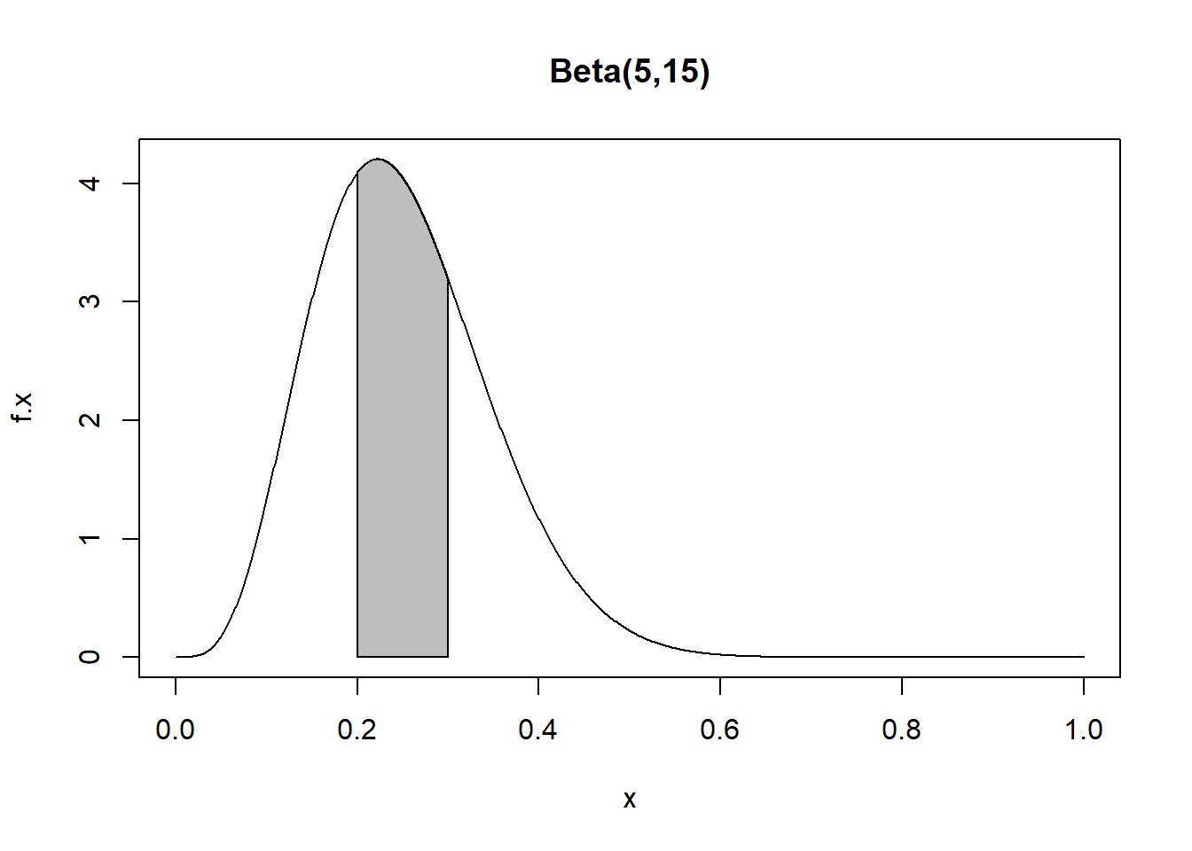
## [1] 0.3910646