Chapter 7 Interval Estimation

7.1 Introduction to Interval Estimation

We have focused on point estimation, i.e. estimating an unknown parameter $\theta$ with a single value $\hat{\theta}$. Now we turn our attention to interval estimation, where we will estimate $\theta$ with a range of plausible values. In fact, the confidence intervals we will consider this semester will all be of the form

$$Statistic \pm Margin \quad of \quad Error$$ where the ‘Statistic’ is a reasonable point estimator (statistic) for the parameter being estimated and the ‘Margin of Error’ is the standard error of the statistic multiplied by a ‘critical value’ based on that statistic’s sampling distribution.

Definition: Let $X_1,\cdots,X_n$ be a random sample from $X_i \sim f(x; \theta), \theta \in \Omega$. Let $0 < \alpha < 1$ be specified (i.e. choose a constant $\alpha$, usually $\alpha=0.05$). Then the interval $(L,U)$ is a $100(1-\alpha)$% confidence interval (CI) for $\theta$ if $$P[\theta \in (L,U)]=1-\alpha$$

This is the frequentist definition, where we consider the parameter $\theta$ to be an unknown constant. The CI ‘captures’ the true value of $\theta$ $100(1-\alpha)$% of the time. It DOES NOT MEAN that there is a $100(1-\alpha)$% chance that the parameter $\theta$ is between the values $L$ and $U$. (This is a very common mistake in interpretation of confidence intervals).

The Bayesian school of statistical thought considers parameters such as $\theta$ to be random variable with their own distributions, rather than unknown constants. Bayesians compute their own interval estimates that are often called credible intervals. The advantage of credible intervals over traditional confidence intervals is that the interpretation is clearer–for a Bayesian $100(1-\alpha)$% credible interval, I can correctly say that there I am $100(1-\alpha)$% confident that $\theta$ is between $L$ and $U$. However, the Bayesian intervals are more difficult to compute than the traditional frequentist intervals. We will concentrate on the traditional intervals for the remainder of this semester.

7.2 Confidence Intervals for Proportions

This is Section 7.3 of your book.

Suppose $X \sim BIN(n,\pi)$. A natural point estimator (it is unbiased!) for $\pi$ is $$\hat{\pi}=\frac{X}{n}$$

When both $n \pi$ and $n (1-\pi)$ are 10 or greater, the distribution of $X$ is well approximated by a normal distribution. $$X \dot{\sim} N(n \pi, \sqrt{n \pi (1-\pi)})$$

We would rather have a formula for our confidence interval for $\pi$ to be based on $\hat{\pi}$, so we need the sampling distribution of $\hat{\pi}$.

$$\mu_{\hat{\pi}}=E(\hat{\pi})=E{\frac{X}{n}}=\frac{1}{n}E(X)=\frac{1}{n}n \pi = \pi$$

$$\sigma^2_{\hat{\pi}}=Var(\hat{\pi})=Var{\frac{X}{n}}=\frac{1}{n^2}Var(X)=\frac{1}{n^2}{n \pi (1-\pi)}=\frac{\pi (1-\pi)}{n}$$

$$\sigma_{\hat{\pi}}=\sqrt{\frac{\pi (1-\pi)}{n}}$$

$$\hat{\pi} \dot{\sim} N(\pi, \sqrt{\frac{\pi (1-\pi)}{n}})$$

We will base our confidence interval formula for $\pi$ on the standard normal distribution $Z \sim N(0,1)$, since the sampling distribution of $\hat{\pi}$ is approximately normal. Our formula will be the statistic plus/minus the margin of error, where the margin of error will be the standard error multiplied by a constant called the critical value. This critical value $z^*$ is chosen such than $100(1-\alpha)$% of the standard normal is between $\pm z^*$.

So the formula for a $100(1-\alpha)$% CI for $\pi$ is:

$$\hat{\pi} \pm z^* \sqrt{\frac{\hat{\pi}(1-\hat{\pi})}{n}}$$

The usual choice is $\alpha=0.05$, leading to a 95% confidence level. The appropriate $z^*=\pm 1.96$. You can find $z^*$ from the normal table or by using invNorm(0.025) and invNorm(0.975)

We can also find critical values with R for 95% confidence or other common choices such as $\alpha=0.10$ or $\alpha=0.01$, leading to 90% or 99% CIs, respectively.

alpha<-c(0.10,0.05,0.01)
qnorm(c(alpha/2,1-alpha/2))

## [1] -1.644854 -1.959964 -2.575829  1.644854  1.959964  2.575829

So we use $z^* = \pm 1.645$ for 90% confidence, $z^*=\pm 1.96$ for 95% confidence, and $z^*=\pm 2.576$ for 99% confidence.

Example: Suppose we have taken a random sample (i.i.d. or simple) of $n=500$ voters, where $X=220$ support Richard Guy, a candidate for political office. The point estimate is $$\hat{\pi}=\frac{220}{500}=0.44$$

ASIDE: Polling companies and news organizations do not use i.i.d. or simple random samples; their sampling designs are more complicated and they compute CIs based on formulas with more complex forms of the standard error. In practice, you would see a minor difference if you recomputed the CI based on our formula.

The interval estimate for 95% confidence is $$\begin{aligned} \hat{\pi} & \pm z^* \sqrt{\frac{\hat{\pi}(1-\hat{\pi})}{n}} \\ 0.44 & \pm 1.96 \sqrt{\frac{0.44(1-0.44)}{500}} \\ 0.44 & \pm 0.0435 \\ & (0.3965,0.4835) \\ \end{aligned}$$

The margin of error of our poll is $\pm 4.35$% and the entire intervals lies below $\pi=0.50$, which is bad news for Richard Guy in his election.

This can be done on the TI-84 calculator with the 1-PropZInterval function under the STAT key.

What will happen to our interval if we change the confidence level from 95% to 99%???

As we’ll see in class, the margin of error increases and the confidence interval will be wider, since the critical value $z^*$ is bigger to capture a larger percentage of the standard normal curve.

What about if the sample size increases, with $\hat{p}$ remaining the same?? (i.e. n=1000 voters, X=440)

As the sample size increase, the margin of error will decrease and the CI will be narrower.

If we want to cut the margin of error in half, what do we need to do to the sample size?

Unfortunately, if $\hat{\pi}$ remains the same, we have to quadruple our sample size to cut the margin of error in half. Doubling the sample size is not sufficient if we want to cut the margin of error in half.

__What about the coverage of the Wald interval?

The problem with the Wald interval based on $\hat{p}$ as described so far is that it depends on the normal approximation to the binomial distribution and that its “coverage” can be less than the stated percentage. In other words, we will capture the true value of a parameter less than 95% of the time.

# let's simulate this
# suppose you guess on a multiple choice exam where each question has 5 choices
# so the true value of the parameter is 1/5, call this theta
theta <- 1/5

# let's randomly generate 10000 samples of size n=100 each and compute the 95% confidence intervals
set.seed(11162021)
samp <- 10000
p.hat <- numeric(samp)
L <- numeric(samp)
U <- numeric(samp)
capture <- logical(samp)
N <- 100

for (i in 1:samp){
  X <- rbinom(n=1,size=N,prob=theta)
  p.hat[i] <- X/N
  L[i] <-  p.hat[i] - 1.96*sqrt(p.hat[i]*(1-p.hat[i])/N)
  U[i] <-  p.hat[i] + 1.96*sqrt(p.hat[i]*(1-p.hat[i])/N)
  capture[i] <- (L[i]< theta & theta < U[i]) # this is TRUE when L<theta<U
}

# is theta containted in CI #i?
table(capture) # TRUE should be 95%, or about 950

## capture
## FALSE  TRUE 
##   701  9299

# but coverage < 95%, so alpha > 5% "liberal"

# graph the first 100
require(ggplot2) # can't really do this graphing in base R
CI <- 1:100
p.hatCI <- p.hat[1:100]
LCI <- L[1:100]
UCI <- U[1:100]
captCI <- capture[1:100]
CIs <- data.frame(CI,p.hatCI,LCI,UCI,captCI)

ggplot(data=CIs,aes(x=CI,y=p.hatCI)) + 
  geom_pointrange(aes(ymin=LCI,ymax=UCI,color=captCI)) +
  geom_hline(yintercept=theta)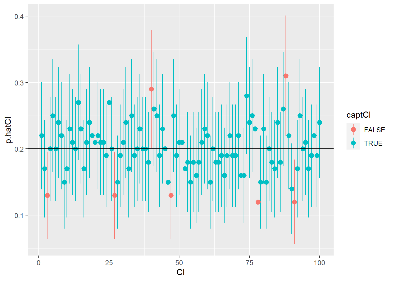

We can consider other estimators for $p$. A biased alternative, due to Wilson, is called the “plus-2/plus-4” estimator, based on adding 2 successes and 2 failures to the sample, thus adding 4 to the overall sample size. The “coverage” of this estimator is better, especially with small sample size $n$. The coverage will exceed the stated percentage and is thus conservative.

$$\tilde{p}=\frac{x+2}{n+4}$$

The confidence interval is:

$$\tilde{p} \pm z^* \sqrt{\frac{\tilde{p}(1-\tilde{p})}{n}}$$

# let's randomly generate 10000 samples of size n=100 each and compute the 95% confidence intervals
# using this estimator, compare to the usual p.hat
set.seed(15112021)
samp <- 10000
p.tilde <- numeric(samp)
L <- numeric(samp)
U <- numeric(samp)
capture <- logical(samp)
N <- 100

for (i in 1:samp){
  X <- rbinom(n=1,size=N,prob=theta)
  p.tilde[i] <- (X+2)/(N+4)
  L[i] <-  p.tilde[i] - 1.96*sqrt(p.tilde[i]*(1-p.tilde[i])/N)
  U[i] <-  p.tilde[i] + 1.96*sqrt(p.tilde[i]*(1-p.tilde[i])/N)
  capture[i] <- (L[i]< theta & theta < U[i]) # this is TRUE when L<theta<U
}

# is theta containted in CI i?
table(capture) # better, coverage > 95%, so alpha < 5% "conservative"

## capture
## FALSE  TRUE 
##   325  9675

7.3 Confidence Intervals for Means

This is section 7.1 of your book.

Suppose we are willing to make some very strong asuumptions about our data. We will assume both normality and that the variance $\sigma^2$ (and standard deviation $\sigma$) is known. So $X \sim N(\mu,\sigma)$ with only $\mu$ unknown.

In this case, we can form a $100(1-\alpha)$% CI for $\mu$ by making some minor adjustments to the formula that we previously used for a proportion.

The format will still be statistic/point estimate $\pm$ margin of error, where the margin of error is $z^* SE$. Instead of using $\sigma_{\hat{\pi}}=\sqrt{\frac{\hat{pi}(1-\hat{\pi})}{n}}$ as the standard error, we use the standard error $\sigma_{\bar{x}}=\frac{\sigma}{\sqrt{n}}$ since $\bar{X} \sim N(\mu, \sigma/\sqrt{n})$.

The $100(1-\alpha)$% CI for $\mu$ is: $$\bar{x} \pm z^* \frac{\sigma}{\sqrt{n}}$$

This is available on the TI calculator as ZInterval.

Example: Suppose it is known that $X$ represents the score obtained on an ACT test, where $X \sim N(\mu, \sigma=5)$, i.e. we know the true standard deviation is $5$. Find a 95% CI for $\mu$ for a sample of size $n=9$ with $\bar{x}=22.0$.

$$\begin{aligned} \bar{x} & \pm z^* \frac{\sigma}{\sqrt{n}} \\ 22.0 & \pm 1.96 \frac{5}{\sqrt{9}} \\ 22.0 & \pm 3.27 \\ & (18.73,25.27) \\ \end{aligned}$$

Confidence Interval for a Single mean $\mu$ with $\sigma$ unknown: The $t$ Interval

However, $\sigma^2$ and hence $\sigma$ are usually unknown to us–it would be strange to have a scenario where $\sigma$ was known but $\mu$ was not. A natural point estimate to use for the unknown $\sigma$ is the sample standard deviation $S$ and instead of basing inference on $$Z=\frac{\bar{X}-\mu}{\sigma/\sqrt{n}} \sim N(0,1)$$ to base it on $$T=\frac{\bar{X}-\mu}{S/\sqrt{n}} \sim ???$$

What is the distribution of $T$? The answer came from the Guinness Bwerey in Dublin, Ireland, during the early 20th century. William Gosset, aka ‘Student’ notice that the sampling distributions for sample means were not quite normal for small samples and he derived the Student’s $t$ distribution.

It turns out that there are a number of distributions that are ‘derived’ from the standard normal distribution that play key roles in statistical methods. Here, I will present but not derive how the $\chi^2$, $t$, and $F$ distributions came about.

Suppose $Z$ is standard normal, i.e. $Z \sim N(0,1)$. It can be shown that the distribution of $Z^2 \sim \chi^2(1)$, that is, a squared $z$-score follows a chi-squared distribution with 1 degree of freedom.

If I have an i.i.d. random sample of size $n$ from $Z \sim N(0,1)$, then by the mgf technique, the distribution of $V=Z_1^2+Z_2^2+\cdots+Z_n^2 \quad$ is $V \sim \chi^2(n)$.

Then (via either the cdf or pdf-to-pdf technique), if $Z \sim N(0,1)$ and $V \sim \chi^2(n)$, then $$T=\frac{Z}{\sqrt{V/n}} \sim t(n)$$ that is, $T$ has a Student’s $t$ distribution with $n$ degrees of freedom.

Also (again (via either the cdf or pdf-to-pdf technique), if $U \sim \chi^2(m)$ and $V \sim \chi^2(n)$, then $$F=\frac{U/m}{V/n} \sim F(m,n)$$ , that is $F$ has a Snedecor’s $F$ distribution with $m$ and $n$ degrees of freedom.

Finally, if $T \sim t(n)$, then $T^2 \sim F(1,n)$.

The $\chi^2$, $t$, and $F$ distributions traditionally appear in statistical tables and are all programmed into R with the usual d-, p-, q- and r- functions.

Let’s look at the $t$ distribution graphically.

require(mosaic)

## Loading required package: mosaic

## 
## The 'mosaic' package masks several functions from core packages in order to add 
## additional features.  The original behavior of these functions should not be affected by this.

## 
## Attaching package: 'mosaic'

## The following object is masked from 'package:purrr':
## 
##     cross

## The following objects are masked from 'package:stats':
## 
##     binom.test, cor, cor.test, cov, fivenum, IQR, median, prop.test,
##     quantile, sd, t.test, var

## The following objects are masked from 'package:dplyr':
## 
##     count, do, tally

## The following object is masked from 'package:Matrix':
## 
##     mean

## The following object is masked from 'package:ggplot2':
## 
##     stat

## The following objects are masked from 'package:base':
## 
##     max, mean, min, prod, range, sample, sum

x<-seq(-3,3,by=0.001)
t5<-dt(x=x,df=5)
t15<-dt(x=x,df=15)
t30<-dt(x=x,df=30)
z<-dnorm(x=x,mean=0,sd=1)
my.colors<-c("blue","red","green","black")
my.key<-list(space = "bottom",
             lines=list(type="l",lty=c(1,1,1,2),col=my.colors),
             text=list(c("t(5)","t(15)","t(30)","z")))    
xyplot(t5+t15+t30+z~x,type="l",lty=c(1,1,1,2),col=my.colors,ylab="Density",
       xlab="X",key=my.key)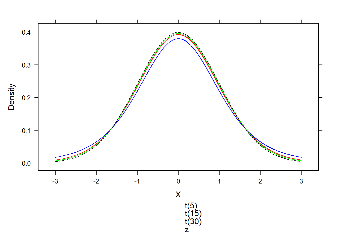

Visually, notice that the $t$ distribution is centered at zero and is bell-shaped, but is flatter and has higher variance than the standard normal. As the degrees of freedom $df \to \infty$, the $t$ distribution converges to the standard normal.

To form a confidence interval for a mean $\mu$ from a random sample of size $n$ from $X \sim N(\mu,\sigma)$ with unknown variance, we will use $s$ and a critical value from the $t$ distribution with $n-1$ df.

The $100(1-\alpha)$% CI for $\mu$ is: $$\bar{x} \pm t^* \frac{\sigma}{\sqrt{n}}$$

Example: I want a 95% CI for $\mu$ for a random sample of size $n=16$ where $\bar{x}=32.4$ and $s=4.4$. To find $t^*$, either use a $t$ table, the invT function on a calculator, or the qt function for quantiles from the $t$ distribution.

On the calculator, use invT(0.025) and invT(0.975), obtaining $t^*=\pm2.131$ if 95% confidence is desired.

# t* for 95%
qt(p=0.975,df=15)         

## [1] 2.13145

$$\begin{aligned} \bar{x} & \pm t^* \frac{s}{\sqrt{n}} \\ 32.4 & \pm 2.131 \frac{4.4}{\sqrt{16}} \\ 32.4 & \pm 2.34 \\ & (30.06,34.74) \\ \end{aligned}$$

This is also available on the TI calculator as TInterval and as part of the output that the R function t.test provides. We’ll consider that function later.

7.4 Bootstrapping

put notes and R code here

7.5 Confidence Intervals for the Difference of Two Means

This is section 7.2 in your book.

Inference can also be done with a confidence interval rather than a hypothesis test. If we want a confidence interval of the difference in means, which is the parameter $\mu_1 - \mu_2$, we have the same issue with the variances as in the hypothesis test.

We can assume equal variance, use $df=n_1+n_2-2$ and the pooled variance.

$$\bar{x_1} - \bar{x_2} \pm t^* \sqrt{s_p^2(\frac{1}{n_1}+\frac{1}{n_2})}$$

Most modern textbooks recommend assuming unequal variances, and instead computing the confidence interval based on not using the pooled variance (i.e. similar to Welch’s $t$-test).

$$\bar{x_1} - \bar{x_2} \pm t^* \sqrt{\frac{s^2_1}{n_1}+\frac{s^2_2}{n_2}}$$

To obtain the critical value $t^*$, one could use the conservative degrees of freedom $df \approx \min(n_1-1,n_2-1)$. This will result in using a critical value larger than you should, and thus the margin of error of the interval would be too large.

It is preferable to use technology with the exact $df$, which can be done on a TI calculator. Go to STAT, then TESTS, and choose 0:2-SampTInt. Use Pooled=No for unequal varainces, which will be the default in R.

Suppose we wanted to form a confidence interval for the difference in means between students in the same course who took a final exam on Monday (the first day of finals week) versus Friday (the last day of finals week).

$$\text{Friday:} \: \: 74 \: 72 \: 65 \: 96 \: 45 \: 62 \: 82 \: 67 \: 63 \: 93 \: 29 \: 68 \: 47 \: 80 \: 87$$

$$\text{Monday} \: \: 100 \: 86 \: 87 \: 89 \: 75 \: 88 \: 81 \: 71 \: 87 \: 97 \: 83 \: 81 \: 49 \: 71 \: 63 \: 53 \: 77 \: 71 \: 86 \: 78$$

scores <- c(76,72,65,96,45,62,82,67,68,93,39,68,47,80,87,
                 100,86,87,89,75,88,81,71,87,97,83,81,49,71,63,50,77)
day <- c(rep("Friday",15),rep("Monday",17))
exam <- data.frame(scores,day)
require(mosaic)
favstats(scores~day,data=exam,type=2)

##      day min Q1 median Q3 max     mean       sd  n missing
## 1 Friday  39 62     68 82  96 69.80000 16.89970 15       0
## 2 Monday  49 71     81 87 100 78.52941 14.33578 17       0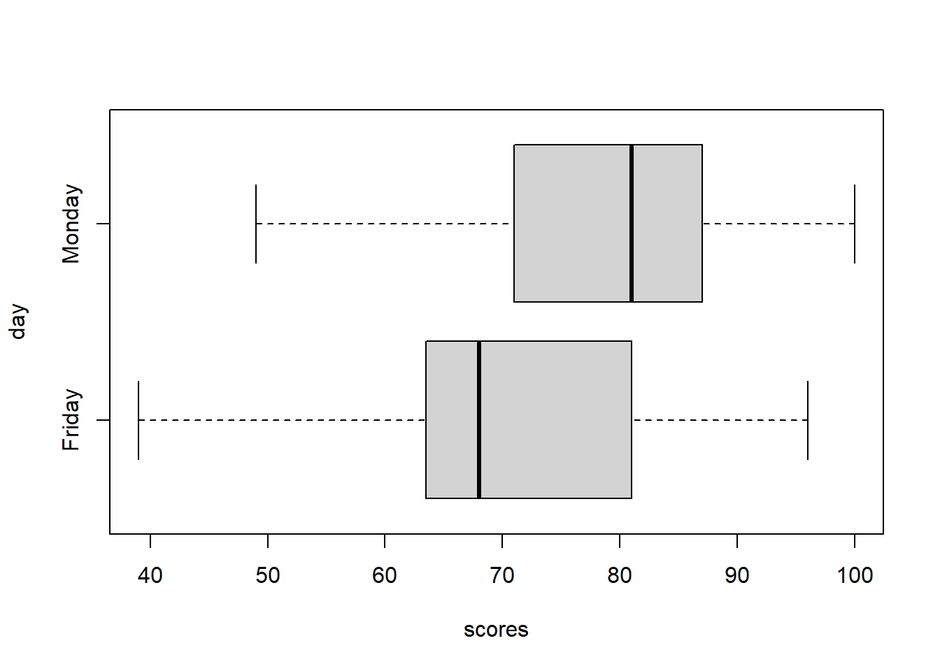

boxplot(scores~day,data=exam,horizontal=TRUE)

Doing this problem by hand assuming unequal variances, my “conservative” df will be 14 and the critical value for a 95% confidence interval is $t^*= 2.145$. So:

$$\bar{x_1} - \bar{x_2} \pm t^* \sqrt{\frac{s^2_1}{n_1}+\frac{s^2_2}{n_2}}$$ $$69.800 - 78.529 \pm 2.145 \sqrt{\frac{16.89970^2}{15} + \frac{14.33578^2}{17}}$$

$$-8.729 \pm 11.968$$

$$(-20.697,3.239)$$

Notice that the null value of zero IS contained in this confidence interval, so we would not conclude that the difference in mean exam scores between the two days is statistically significant. We do not have enough evidence to defend such a claim.

With R:

t.test(scores~day,data=exam) # assumes unequal variances, does not use pooled variance

## 
##  Welch Two Sample t-test
## 
## data:  scores by day
## t = -1.5646, df = 27.664, p-value = 0.129
## alternative hypothesis: true difference in means between group Friday and group Monday is not equal to 0
## 95 percent confidence interval:
##  -20.164445   2.705622
## sample estimates:
## mean in group Friday mean in group Monday 
##             69.80000             78.52941

# t.test(scores~day,data=exam,var.equal=TRUE) # assumes equal variances, uses pooled variance

Notice the difference in the calculation is due to R using $df=27.664$ rather than our conservative estimate $df=14$.