Chapter 5 Distributions of Functions of Random Variables
5.1 Functions of One Random Variable
We will very often wish to determine the pdf of a transformation of a random variable \(X\). For example, we wish to know the pdf of \(Y\), where \(Y=2X-5\) or \(Y=X^2\) or \(Y=\sqrt{X}\) or \(Y=\ln X\) or similar.
There are 3 major methods for determining \(f_Y(y)\).
The cdf method or distribution function technique
The pdf-to-pdf or change of variable or Jacobian method (usually my favorite)
The mgf method based on moment-generating functions that we’ll study later.
Let’s describe the cdf method and then use it on a simple example.
Let \(X\) be a continuous random variable with pdf \(f(x)\) and cdf \(F(x)\). Let \(Y=u(X)\), where \(u\) is a one-to-one function. Our goal is to find \(f_Y(y)\), the pdf of \(Y\).
In this method, we first find \(F_Y(y)\), the cdf of \(Y\). Once we have found the cdf of \(Y\), we obtain the pdf of \(Y\) by taking the first derivative of the cdf.
\[ \begin{aligned} F_Y(y) & = P(Y \leq y) \\ & = P(u(X) \leq y) \\ & = P(X \leq u^{-1}(y)) \\ & = F_X(u^{-1}(y)) \\ \end{aligned} \]
So \[ \begin{aligned} f_Y(y) & = \frac{dF_Y(y)}{dy} \\ & = F'_Y(y) \\ \end{aligned} \]
Example: Let \(X\) have pdf \(f(x)=2x, 0 \leq x\leq 1\) and zero elsewhere. Let \(Y=X^2\). Notice that this function is one-to-one over the interval \([0,1]\) and the support for \(Y\) is \([0,1]\).
\[ \begin{aligned} F_Y(y) & = P(Y \leq y) \\ & = P(X^2 \leq y) \\ & = P(X \leq \sqrt{Y}) \\ & = F_X(\sqrt{Y}) \\ & = \int_0^{\sqrt{Y}} 2x \quad dx \\ & = x^2|_0^{\sqrt{Y}} \\ & = y \\ \end{aligned} \] So the cdf of \(Y\) is \[F_Y(y)=0, y<0; F_Y(y)=y, 0 \leq y \leq 1; F_Y(y)=1, y>1\]
Taking the derivative, clearly \(f_Y(y)=1, 0 \leq y \leq 1\) and zero otherwise. You should recognize this as the pdf of a continuous uniform \[Y \sim UNIF(0,1)\]
In my opinion, the theory behind the pdf-to-pdf method is a bit more difficult that for the cdf method, but it is often easier to compute in practice. An advantage of the pdf-to-pdf method is that we will directly compute the pdf for the transformation \(Y\) without the middle step of finding the cdf of \(Y\).
Again, let \(X\) be a continuous random variable with pdf \(f(x)\) and cdf \(F(x)\). Let \(Y=u(X)\), where \(u\) is a one-to-one function. Let \(X=w(y)\) be the inverse function. Our goal is to find \(f_Y(y)\), the pdf of \(Y\).
Theorem: Let \(f(x)\) be the pdf of continuous random variable \(X\). If the function given by \(y=u(x)\) is differentiable and is either monotonically increasing or decreasing for all values where \(f(x)>0\), then the equation \(y=u(x)\) can be solved for \(x\) to yield \(x=w(y)\). Then, the pdf of \(Y=u(X)\) is given as:
\[g(y)=f[w(y)] \cdot |w'(y)|\] provided that \(u'(x) \neq 0\). Elsewhere, \(g(y)=0\).
Proof: I will provide the proof for the case that \(y=u(x)\) is an increasing function.
(FIGURE-will draw in class)
As can be seen in the figure, \(X\) must take on a value between \(w(a)\) and \(w(b)\) when \(Y\) takes on a value between \(a\) and \(b\)). Now perform the change of variable \(y=u(x)\) or equivalently \(x=w(y)\) in the above integral. Thus \(dx=w'(y) dy\) and we obtain the following.
\[ \begin{aligned} P(a < Y < b) & = P[w(a) < X < w(b)] \\ & = \int_{w(a)}^{w(b)} f(x) dx \\ & = \int_a^b f[w(y)] w'(y) dy \\ \end{aligned} \]
This integral, provided \(w'(y)\) exists, is the probability density function for \(Y\), and thus
\[g(y)=f[w(y)] \cdot w'(y)\]
The proof is similar when \(y=u(x)\) is decreasing except \(g(y)=-f[w(y)] \cdot w'(y)\). Since \(w'(y)\) is positive when \(y=u(x)\) is increasing and \(w'(y)\) is negative when \(y=u(x)\) is decreasing. We combine the two cases as \[g(y)=f[w(y)] \cdot |w'(y)|\]
Example: First, let’s re-do the simple example from earlier.
Let \(X\) have pdf \(f(x)=2x, 0 \leq x\leq 1\) and zero elsewhere. Let \(Y=X^2\). Notice that this function is one-to-one over the interval \([0,1]\) and the support for \(Y\) is \([0,1]\).
Notice that since \(Y=X^2\), that \(X=+\sqrt{Y}\) and \(w(y)=\sqrt{y}\).
\[ \begin{aligned} g(y) & = f[w(y)] \cdot w'(y) \\ & = 2\sqrt{y} \cdot |\frac{1}{2}y^{-1/2}| \\ & = 1, \quad 0 \leq y \leq 1 \\ & = 0, \quad otherwise \\ \end{aligned} \]
Obviously, we should get the same answer with either method, and we do, showing that \(Y \sim UNIF(0,1)\).
Example: Let’s try a slightly more difficult example. Let our random variable \(X\) be given by \[f(x)=e^{-x}, x \geq 0\] and zero otherwise. Find the pdf for \(Y=\sqrt{X}\).
Solution: The equation \(y=\sqrt{x}\) has inverse \(x=y^2\), yielding \(w'(y)=\frac{dx}{dy}=2y\). Since the support of \(X\) is \([0,\infty)\), the support of \(Y=\sqrt{X}\) will also be \([0,\infty]\).
\[ \begin{aligned} g(y) & = f[w(y)] \cdot w'(y) \\ & = e^{-y^2} \cdot |2y| \\ & = 2ye^{-y^2}, \quad y>0 \\ & = 0, \quad otherwise \\ \end{aligned} \]
Suppose I want to find \(P(1 < X< 4)\) and \(P(1 < Y < 2)\). We have:
\[ \begin{aligned} P(1 < X < 4) & = \int_1^4 f(x) dx \\ & = \int_1^4 e^{-x} dx \\ & = -e^{-x}|_1^4 \\ & = e^{-1}-e^{-4} \\ & \approx 0.35 \\ P(1 < Y < 2) & = \int_1^2 g(y) dy \\ & = \int_1^2 2y e^{-y^2} dy \\ \end{aligned} \]
That integral is easy to solve if you make the substition \(u=y^2\), thus \(du=2y dy\), and you end up with the same integral as before
\[ \begin{aligned} & = \int_1^2 2y e^{-y^2} dy \\ & = \int_1^{2^2} e^{-u} du \\ & \approx 0.35 \\ \end{aligned} \]
## 0.3495638 with absolute error < 3.9e-15curve(f.x,from=0, to=5)
abline(v=0)
abline(h=0)
tt<-seq(from=1,to=4,length=100)
dtt<-f.x(tt)
polygon(x=c(1,tt,4),y=c(0,dtt,0),col="gray")
title("P(1<X<4)")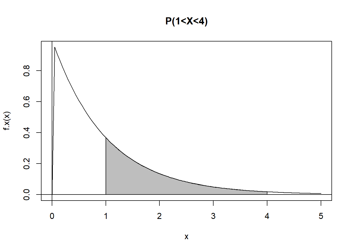
## 0.3495638 with absolute error < 3.9e-15curve(g.y,from=0, to=5)
abline(v=0)
abline(h=0)
tt<-seq(from=1,to=2,length=100)
dtt<-g.y(tt)
polygon(x=c(1,tt,2),y=c(0,dtt,0),col="gray")
title("P(1<Y<2)")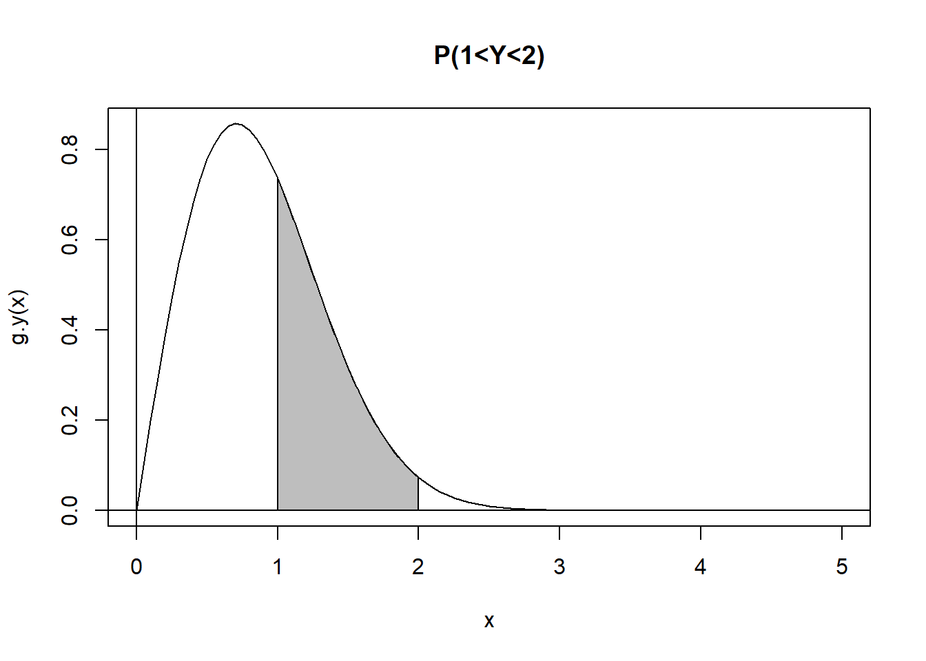
\(X\) is a special case of the exponential distribution and that \(Y\) is a special case of the Weibull distribution.
5.2 Transformations of Two Random Variables
suppose that we have two random variables \(X_1\) and \(X_2\) with joint pdf \(f(x_1,x_2)\). If we have one-to-one transformations \(Y_1=u_1(x_1)\), \(Y_2=u_2(x_2)\) where \(X_1=w_1(y_1)\) and \(X_2=w_2(y_2)\), then define the Jacobian of the transformation to be the determinant of the partial derivatives:
\[ J = \left| \begin{array}{cc} \frac{\partial w_1}{\partial y_1} & \frac{\partial w_1}{\partial y_2} \\ \frac{\partial w_2}{\partial y_1}& \frac{\partial w_2}{\partial y_2} \end{array} \right| \]
Then the joint pdf of \(Y_1\) and \(Y_2\) is obtained as: \[g(y_1,g_2)=f[w_1(y1,y2),w_2(y1,y2)] \cdot |J|\]
If one desires the marginal pdf of either \(Y_1\) or \(Y_2\), it is obtained by ‘integrating out’ the other variable.
Problem: Let’s apply the pdf-to-pdf technique to our example involving the sum of two uniform random variables.
\(X_1\) and \(X_2\) are i.i.d. random varaibles from \(X \sim UNIF(0,1)\), so \(f(x)=1, 0 < x < 1\). We want the distribution of \(Y_1=X_1+X_2\). This technique demands that we define a second transformation variable as well. We will choose \(Y_2=X_2\).
Solving those equations for \(X_1\) and \(X_2\), these choices for the transformation variables yields \[w_1(y_1,y_2)=x_1=y_1-y_2, w_2(y_1,y_2)=x_2=y_2\]
One of the most difficult parts of this method is to correctly define the support space of the transformation.
\[\mathcal{S}_X=\{(x_1,x_2): 0 < x_1 <1, 0 < x_2 <1 \} \to \mathcal{S}_Y=\{(y_1,y_2): 0 < y_1 < 2, 0 < y_2 < 1, y_2 < y_1 \}\]
I’ll draw the pitcure of this space in class; \(\mathcal{S}_X\) is a unit square but \(\mathcal{S}_Y\) is a parallelogram with vertices \((0,0),(1,0),(1,1),(2,1)\).
Now we will find the Jacobian, recalling that \(w_1(y_1,y_2)=y_1-y_2\) and \(w_2(y_1,y_2)=y_2\).
\[ \begin{aligned} J = & \left| \begin{array}{cc} \frac{\partial w_1}{\partial y_1} & \frac{\partial w_1}{\partial y_2} \\ \frac{\partial w_2}{\partial y_1}& \frac{\partial w_2}{\partial y_2} \end{array} \right| = & \left| \begin{array}{cc} 1 & -1 \\ 0 & 1 \end{array} \right| = & 1 \\ \end{aligned} \]
Since \(X_1\) and \(X_2\) are i.i.d., then \(f(x_1,x_2)=f(x_1) \cdot f(x_2)= 1 \cdot 1 = 1\).
So \[g(y_1,y_2)=g(y_1,g_2)=f[w_1(y1,y2),w_2(y1,y2)] \cdot |J|= 1 \cdot 1 = 1, (y_1,y_2) \in \mathcal{S}_Y\]
Remember, we actually want the marginal pdf of \(Y_1\), not the joint pdf that includes the unneeded and unwanted variable \(Y_2\). So we will ‘integrate’ \(Y_2\) out so \(g(y_1)=\int_{\mathcal{S_Y}} g(y_1,y_2) dy_2\).
I’ll draw the picture of \(\mathcal{S}_Y\) in class, but it’s a parallelogram and we have to break into 2 cases.
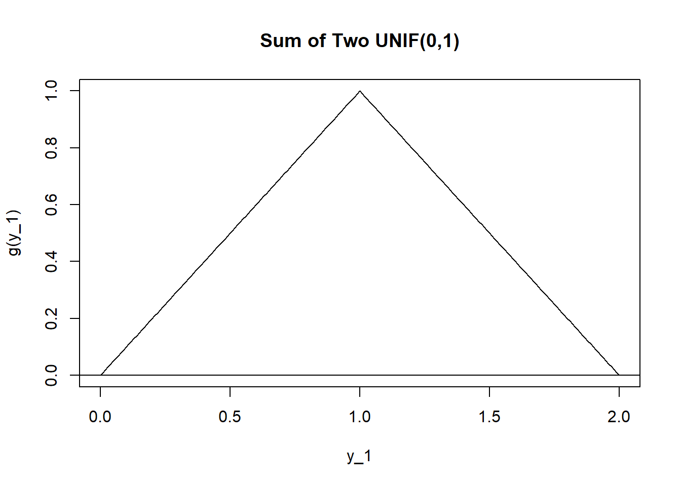
Case I: If \(0 < y_1 < 1\), then \[ \begin{aligned} g(y_1) = & \int_0^{y_1} 1 dy_2 \\ = & y_2|_0^{y_1} \\ = & y_1 \\ \end{aligned} \]
Case II: If \(1 \leq y_1 < 2\), then \[ \begin{aligned} g(y_1) = & \int_{y_1-1}^1 1 dy_2 \\ = & y_2|_{y_1-1}^1 \\ = & 1-(y_1-1) \\ = & 2-y_1 \\\end{aligned} \]
Hence, the distribution of \(Y_1=X_1+X_2\) is not uniform (although \(X_1\) and \(X_2\) were), but triangular. Basically, when we add two \(UNIF(0,1)\) random variables together, we can get a sum anywhere between 0 and 2 but are more likely to get values near 1 and less likely to get values near 0 or 2.
This is very similar to when we considered rolling 2 dice (i.e. discrete uniform random variables) and noticed that rolling totals like 6, 7, or 8 was more likely that totals like 2,3,11,12.
5.4 The Moment-Generating Function Technique
We are very often interested in the distribution of either a sum of two (or more) random variables and/or the distribution of the mean of a sample.
If \(X\) and \(Y\) are random variables, then:
\(E(X+Y)=E(X)+E(Y)\)
\(E(XY)=E(X)\cdot E(Y)\) if \(X\) and \(Y\) are independent
\(Var(X+Y)=Var(X)+Var(Y)+2 Cov(X,Y)\) (If \(X\) and \(Y\) are independent, the covariance term is equal to zero)
We also need some results about moment generating functions.
If \(Y=aX+b\) (i.e. \(Y\) is a linear transformation), then \(M_Y(t)=M_{aX+b}(t)=e^{bt}M_X(at)\)
If \(X\) and \(Y\) are independent and \(S=X+Y\), then \(M_S(t)=M_X(t)\cdot M_Y(t)\)
Proof: \(M_S(t)=E(e^{tS})=E(e^{t(X+Y)})=E(e^{tx} \cdot e^{ty})=M_X(t) \cdot M_Y(t)\)
If \(X_1, X_2, \cdots, X_n\) are independent random variables with mgfs \(M_{X_i}(t)\), respectively, and \(Y=\sum_{i=1}^n a_i X_i\), then \(M_Y(t)=\prod_{i=1}^n M_{X_i}(a_i t)\)
If \(X_1, X_2, \cdots, X_n\) are independent random variables such that all marginal distributions are the same, i.e. \(f\) is the common pdf for each \(X_i\), then these variables are said to be i.i.d. (independently and identically distributed).
If \(Y\) is the sum of \(n\) i.i.d. random variables \(X_i\), then \(M_Y(t)=[M_X(t)]^n\).
The so-called moment generating function technique is often useful for determining the distributon of a sum of independent random variables. As I’ve said in class, this technique is typically either very easy or totally impossible. The idea is to find the mgf of the sum; when we are lucky, this mgf will be instantly recognizable as being from a familiar distribution family. When we are less lucky, the mgf will be unfamiliar and another technique will be necessary.
Example: Let \(X_1,X_2,\cdots,X_n\) be independent random variables such that \(X_i \sim POI(\lambda_i)\). Notice this is NOT i.i.d., as each \(X_i\) has a potentially different value for the \(\lambda_i\) parameter. If \(Y=\sum X_i\), what is the pdf of \(Y\)?
\[ \begin{aligned} M_Y(t)= & M_{X_1}(t) \cdot M_{X_2}(t) \cdot \cdots \cdot M_{X_n}(t) \\ = & e^{-\lambda_1+\lambda_1 e^t} \cdot e^{-\lambda_2+\lambda_2 e^t} \cdot \cdots \cdot e^{-\lambda_n+\lambda_n e^t} \\ = & e^{-\sum \lambda_i +(\sum \lambda_i)e^t} \\ \end{aligned} \]
We recognize this as the mgf of a Poisson random variable with parameter \(\sum \lambda_i\). Hence \(Y ~ POI(\lambda_i)\).
Distribution families such as the Poisson, normal, and binomial are unusual in that the distribution of a sum of independent random variables from that family is another random variable from that same family. In general, this is not true.
Let’s consider an example from the uniform distribution.
Problem: Let \(X_1\) and \(X_2\) be i.i.d. \(X_i \sim UNIF(0,1)\). What is the distribution of \(Y=X_1+X_2\)?
Let’s try the mgf technique, recalling that \(M_{X_i}(t)=\frac{e^t-1}{t}\).
\[M_y(t)=[\frac{e^t-1}{t}]^2\]
Unfortunately, the mgf of \(Y\) does not fit the form for the uniform distribution or any of the other probability distributions that we have studied. Since we have no method that works in general for recovering the pdf \(g(y)\) from its mgf \(M_Y(t)\), the mgf technique fails us.
5.5 Random Functions Associated With The Normal Distribution
Example: Let \(X_1,X_2,\cdots,X_n\) be i.i.d. random variables \(X_i \sim N(\mu,\sigma)\); that is, a random sample of size \(n\) from the same normal distribution. Find the distribution of \(S=\sum X_i\).
Again, apply the mgf technique.
\[ \begin{aligned} M_X(t)= & e^{\mu t + \sigma^2 t^2/2} \\ M_S(t)= & [e^{\mu t + \sigma^2 t^2/2}]^n \\ = & [e^{\mu t} \cdot e^{\sigma^2 t^2/2}]^n \\ = & e^{n \mu t} \cdot e^{n \sigma^2 t^2/2} \\ = & e^{n \mu t + n \sigma^2 t^2/2} \\ \end{aligned} \]
Hence, \(S \sim N(n \mu, \sqrt{n \sigma^2})\), or \(E(S)=n \mu_X\), \(Var(S)=n \sigma^2_X\), and \(SD(S)=\sigma_X \sqrt{n}\).
Now let \(\bar{X}=\frac{S}{n}\). Notice that \(\bar{X}\) is a random variable! As you will see, the distribution of the mean of a sample of independent random variables is very important in statistics. The distribution of \(\bar{X}\) is called the sampling distribution for the sample mean.
\[\mu_{\bar{X}}=E(\bar{X})=E(\frac{S}{n})=\frac{1}{n}E(S)=\frac{1}{n}n \mu_X=\mu_X\]
\[\sigma^2_{\bar{X}}=Var(\bar{X})=Var(\frac{S}{n})=\frac{1}{n^2}Var(S)=\frac{1}{n^2}n \sigma^2_X=\frac{\sigma^2_X}{n}\]
\[\sigma_{\bar{X}}=\sqrt{\frac{\sigma^2_X}{n}}=\frac{\sigma_X}{\sqrt{n}}\]
The standard deviation of the sampling distribution is usually called the standard error.
5.6 The Central Limit Theorem
The single most important theorem in statistics (I think it should be called The Fundamental Theorem of Statistics) is the Central Limit Theorem. I will state and prove slightly differently than the text. My prove assumes that the moment generating funciton \(M(t)\) exists for \(f(x)\). Without this assumption, a more difficult proof involving characteristic functions (beyond the scope of this class) is needed, where the characteristic function is \[\phi(t)=E(e^{itx})\]
Central Limit Theorem: If \(X_1,X_2,\cdots,X_n\) is a random sample from \(X \sim f(x)\) with finite mean \(\mu\) and finite variance \(\sigma^2>0\), then \[Z_n=\frac{\bar{x}-\mu}{\sigma/\sqrt{n}}=\frac{\sum X_i-n\mu}{\sqrt{n}\sigma} \overset{D}{\to} N(0,1)\] as \(n \to \infty\).
Proof: Let \(m(t)\) denote the MGF of \(X-\mu\). Note that \(m(t)=E(e^{t(x-\mu)})=e^{-\mu t}M(t)\), \(m(0)=1\), \(m'(0)=E(X-\mu)=0\), and \(m''(0)=E(X-\mu)^2=\sigma^2\).
Recall that if \(f\) is a function and \(f(x)=\sum a_n x^n\) for all \(x\) in an open interval \((-r,r)\), then \(f\) can be represented by the Taylor series about c \[f(x)=f(0)+f'(0)(x-c)+\frac{f''(0)}{2!}(x-c)^2+\cdots\]
The special case of a Taylor series where \(c=0\) is called a Maclaurin series. So \(m(t)\) may be represented as \[m(t)=m(0)+m'(0)t+\frac{m''(0)}{2!}t^2+\cdots\]
Also recall that a Taylor Series may be expressed as \[f(x)=f(a)+\frac{f'(a)(x-a)}{1!}+\frac{f''(a)(x-a)^2}{2!}+\cdots+\frac{f^{(n)}(a)(x-a)^n}{n!}+R_n\] where \[R_n=\frac{f^{(n+1)}(\xi)(x-a)^{n+1}}{(n+1)!}\] is called the Taylor series remainder for \(\xi\) between \(x\) and \(a\).
Hence, for \(0< \xi < t\), \[ \begin{aligned} m(t) & = m(0)+m'(0)+R_n \\ & = 1+0+\frac{m''(\xi)(t-0)^2}{2!} \\ & = 1+\frac{\sigma^2 t^2}{2}+\frac{(m''(\xi)-\sigma^2)t^2}{2} \\ \end{aligned} \]
Let \[Z_n=\frac{\bar{x}-\mu}{\sigma/\sqrt{n}}\]
So \[ \begin{aligned} M_{Z_n}(t) & = E[e^{t(\frac{\bar{x}-\mu}{\sigma/\sqrt{n}})}]\\ & = E[e^{t/n(\frac{\sum x_i - n\mu}{\sigma/\sqrt{n}})}] \\ & = E[e^{\frac{t}{\sigma\sqrt{n}}(x_1-\mu+x_2-\mu+\cdots+x_n-\mu)}] \\ & = E[e^{\frac{t}{\sigma\sqrt{n}}(x_1-\mu)} \cdot e^{\frac{t}{\sigma\sqrt{n}}(x_2-\mu)} \cdot \cdots \cdot e^{\frac{t}{\sigma\sqrt{n}}(x_n-\mu)}] \\ & = m_{x_1}(\frac{t}{\sigma\sqrt{n}}) \cdot m_{x_2}(\frac{t}{\sigma\sqrt{n}}) \cdot \cdots \cdot m_{x_n}(\frac{t}{\sigma\sqrt{n}}) \\ & = [m(\frac{t}{\sigma\sqrt{n}})]^n \\ & = [1+\frac{\sigma^2(t/\sigma\sqrt{n})^2}{2}+\frac{(m''(\xi)-\sigma^2)(t/\sigma\sqrt{n})^2}{2}]^n \\ & = [1+\frac{t^2/2}{n}+\frac{(m''(\xi)-\sigma^2)t^2/2\sigma^2}{n}]^n \\ \end{aligned} \]
Now, using the fact that \[\lim_{n \rightarrow \infty} (1+\frac{b}{n}+\frac{\varphi(n)}{n})^{cn}=e^{bc}\] if \[\lim_{n \rightarrow \infty}\frac{\varphi(n)}{n}=0\]
Here, \(b=t^2/2\), \(c=1\), and \(\varphi(n)=(m''(\xi)-\sigma^2)(t^2/2\sigma^2)\).
Thus, \[\lim_{n \rightarrow \infty} m(t)=e^{t^2/2}\] for all \(t\). But we recognize \(e^{t^2/2}\) as the moment generating function of the standard normal distribution. This means that the limiting distribution of \[Z_n=\frac{\bar{x}-\mu}{\sigma/\sqrt{n}}\] is \(N(0,1)\) or \[Z_n \overset{D}{\to} Z \sim N(0,1)\]
Applying the Central Limit Theorem
Example #1: Suppose it is known that \(X \sim N(175,8)\) where \(X\) is the height of adult men, in cm. Find \(P(\bar{X} > 183)\) for samples of size \(n=25\).
We know the sampling distribution of \(\bar{X}\) is \(\bar{X} \sim N(175,8/5)\). Also, \[Z=\frac{\bar{x}-175}{8/5} \sim N(0,1)\].
\[P(\bar{X} > 183)=P(Z > \frac{183-175}{8/5}) = P(Z > 5)\]
So the probability of finding a sample of \(n=25\) men with an average height of more than 180 cm is essentially zero. You won’t even find \(Z=5.00\) on the normal table. You could use normalcdf(180,1E99,175,8/5) on a TI-calculator or
## [1] 0.0000002866516## [1] 0.0000002866516Compare this to the probability of finding a single man taller than 183 cm. \(P(X > 183)=P(Z > \frac{183-175}{8}) = P(Z >1)=1-.8413=0.1587\) via table, or normalcdf(183,1E99,175,8) on the calculator or
## [1] 0.1586553## [1] 0.1586553In general, averages are less variable than individual observations.
height<-seq(150,200,by=0.001)
f.xbar<-dnorm(x=height,mean=175,sd=8/5)
f.x<-dnorm(x=height,mean=175,sd=8)
plot(f.xbar~height,type="l",lty=2,col="blue",ylab="Density",
       xlab="Height (cm) ")
points(f.x~height,type="l",lty=1,col="red")
abline(v=183,h=0)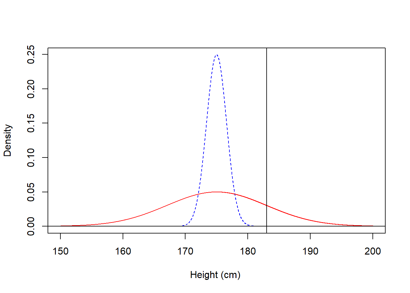
The area under the red dotted curve (which represents individual men) to the right of \(X=183\) cm is about 15%, while the corresponding area under the blue solid curve (which represents \(\bar{X}=183\) cm for samples of 25 men) is essentially 0%.
Example #2: The beauty of the Central Limit Theorem is that even when we sample from a population whose distribution is either unknown or is known to be some heavily skewed (and very non-normal) distribution, the sampling distribution of the sample mean \(\bar{X}\) is approximately normal when \(n\) is ‘large’ enough. Often \(n > 30\) is used as a Rule of Thumb for when the sampling distribution will be large enough.
A nice online demonstration of this can be found at (http://www.lock5stat.com/statkey/index.html). At this site, go to Sampling Distribution: Mean link (about the middle of the page or directly at http://www.lock5stat.com/statkey/sampling_1_quant/sampling_1_quant.html). In the upper left hand corner, change the data set to Baseball Players-this is salary data for professional baseball players in 2012. On the right hand side, you see that the population is heavily right-skewed due to a handful of players making HUGE salaries.
You can choose samples of various sizes–the default is \(n=10\) and generate thousands of samples. The sample mean \(\bar{X}\) is computed for each sample and the big graph in the middle of the page is the sampling distribution. Notice what happens to the shape of this distribution, along with the mean and the standard error of the sampling distribution.
The original population of \(n=855\) players is heavily skewed and non-normal with mean \(\mu=3.439\) million dollars (wow!) and \(\sigma=4.698\) million. I will take 10000 samples, each of size \(n=50\).

The mean of the sampling distribution of \(\bar{X}\) is \(3.444\), which is very close to \(\mu\) for the population.
The standard error of the sampling distribution is \(0.636\). Theoretically, it should be \(\sigma_{\bar{X}}=\frac{\sigma}{\sqrt{n}}=\frac{4.698}{\sqrt{50}}=0.664\), again very close.
The shape is approximately normal (although a bit of skew is still visible).
5.7 Approximations for Discrete Distributions
Under certain conditions, the binomial random variable is approximately normal.
If \(X_n \sim BIN(n,\pi)\), where \(X_n=\sum_{i=1}^n Y_i\) and each \(Y_i \overset{i.i.d.}{\sim} BIN(1,\pi)\).
We know \(E(Y_i)=\pi\) and \(Var(Y_i)=\pi (1-\pi)\). Since \(X_n=n \bar{Y}\), by CLT, then we know if \(n\) is ‘large’,
\(X_n\) is approximately normal
\(E(X_n)=E(n \bar{Y})=n \pi\)
\(Var(X_n)=Var(n \bar{Y})=n \pi (1-\pi)\) and \(SD(X_n)=\sqrt{n \pi (1-\pi)}\)
That is, \[\frac{X_n - n \pi}{\sqrt{n \pi (1-\pi)}} \overset{D}{\rightarrow} N(0,1)\]
The usual Rule of Thumb is that the normal approximation to the binomial holds when both \(n \pi\) and \(n (1-\pi)\) are 10 or greater.
# Xn ~ BIN(200,0.1), meets the Rule of Thumb
x <- seq(0, 40, by = 1)
fx.bin <- dbinom(x = x, size = 200, prob = 0.1)
plot(fx.bin ~ x, type = "h", col = "blue", main = "Normal Approx. to Binomial is OK")
# Xn ~ BIN(25,0.1), does not meet the Rule of Thumb
x <- seq(0, 10, by = 1)
fx.bin <- dbinom(x = x, size = 25, prob = 0.1)
plot(fx.bin ~ x, type = "h", col = "red", main = "Normal Approx. to Binomial is not OK")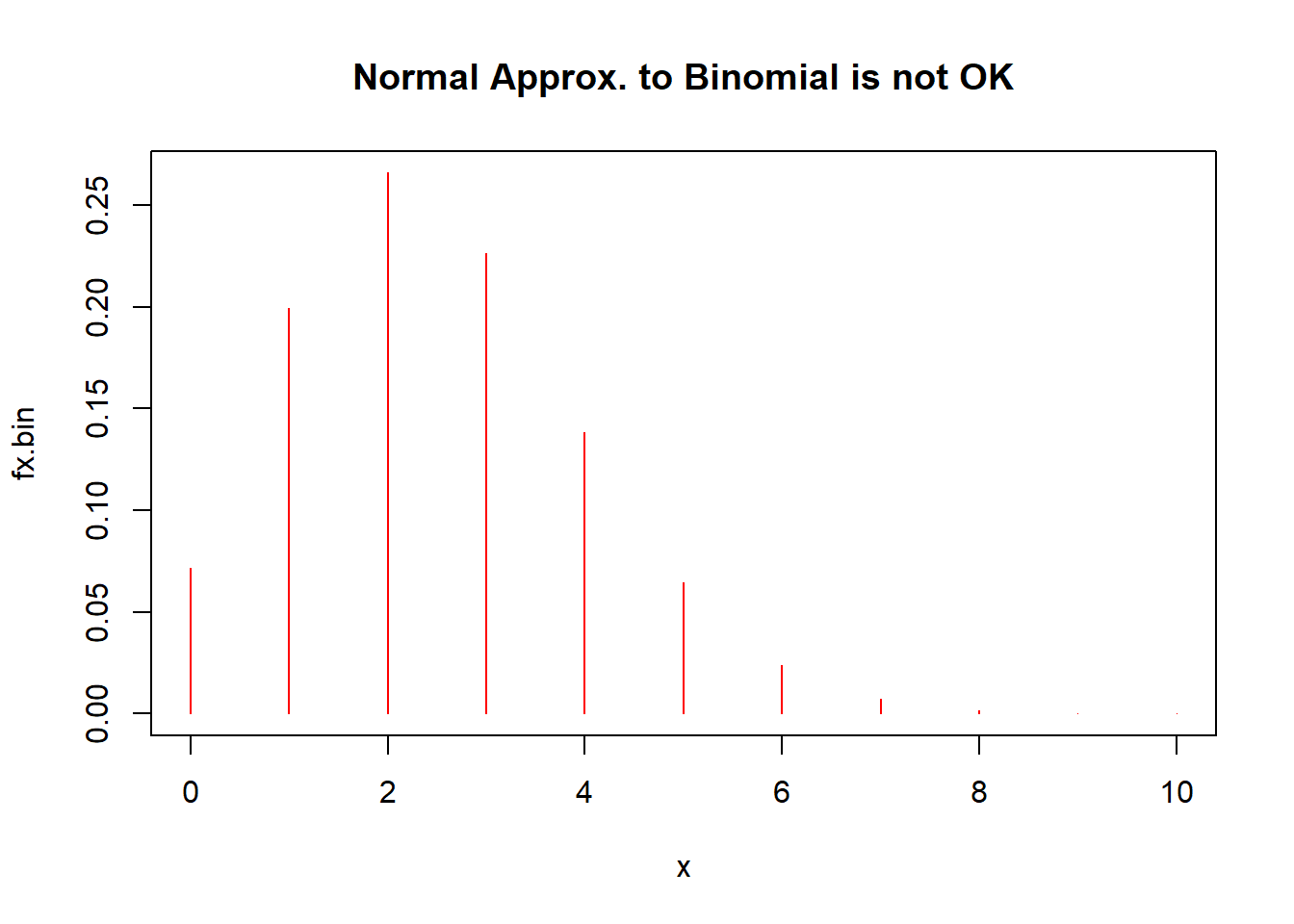
Suppose I have \(X \sim BIN(500,0.4)\) and I want to find \(P(200 \leq X \leq 210)\). With technology, we can compute this probability.
## [1] 0.3481487Utilizing the normal approximation to the binomial, \[X \dot{\sim} N(200,\sqrt{120})\]
#normal approximation without continuity correction
pnorm(q=210,mean=200,sd=sqrt(120))-pnorm(q=200,mean=200,sd=sqrt(120))
## [1] 0.3193448When approximating a discrete distribution such as the binomial with a continuous distribution such as the normal, we should utilize the continuity correction factor. If \(X\) is binomial and \(a,b\) are integers, use \[P(a \leq X \leq b) = P(a-0.5 \leq X \leq b+0.5)\]
Why? When you use the binomial, \(P(X=a)\) is found by directly evaluating the pdf \(f(x)\) with \(x=a\). But using the normal, \(P(X=a)=0\). We can approximate \(P(X=a)\) by using \(P(a-0.5 \leq X \leq a+0.5)\), i.e. finding the area under the normal curve in a neighboorhood of \(a \pm 0.5\).
##normal approximation with continuity correction
pnorm(q=210.5,mean=200,sd=sqrt(120))-pnorm(q=199.5,mean=200,sd=sqrt(120))
## [1] 0.3493011You can see the improvement!
5.8 Chebyshev’s Inequality and Convergence In Probability
I will start by stating and proving Markov’s Inequality, then showing that Chebyshev’s Inequality is a special case of it.
Markov’s Inequality: Let \(u(X)\) be some nonnegative function of random variable \(X\). If \(E[u(X)]\) exists, then for all positive constants \(c\), \[P[u(X) \geq c] \leq frac{E[u(X)]}{c}\]
Proof: (I will do for discrete \(X\), the proof is similar if \(X\) is continuous)
Let \(A=\{x: u(x) \geq c \}\) and \(f(x)\) be the p.m.f. of \(X\). Then \[ \begin{aligned} E[u(X)] & = \sum_{x \in S} u(x) f(x) \\ & = \sum_{x \in A} u(x) f(x) + \sum_{x \in A^c} u(x) f(x) \\ \end{aligned} \]
Since both summations are nonnegative since \(u(x) \geq 0\) and \(f(x) \geq 0\), and if \(x \in A\), then \(u(x) \geq c\), \[ \begin{aligned} E[u(X)] & \geq \sum_{x \in A} u(x) f(x) \\ & \geq \sum_{x \in A} c f(x) \\ & \geq c P(A) \\ & \geq c P[u(x) \geq c] \\ P[u(x) \geq c] & \leq \frac{E[u(X)]}{c} \\ \end{aligned} \]
As you will see, Chebyshev’s Inequality is a special case of Markov’s Inequality.
Chebyshev’s Inequality: For any random variable \(X\) with mean \(\mu\) and finite variance \(\sigma^2\), then for any \(k > 0\), \[P(|X-\mu| \geq k \sigma) \leq \frac{1}{k^2} (upper bound)\] \[P(|X-\mu| < k \sigma) \geq 1-\frac{1}{k^2} (lower bound)\]
Proof: Take Markov’s Inequality, \[P[u(X) \geq c] \leq \frac{E[u(X)]}{c}\] and let \(u(x)=(X-\mu)^2\) and \(c=k^2 \sigma^2\). Then \[ \begin{aligned} P[(X-\mu)^2 \geq k^2 \sigma^2] & \leq \frac{E[(X-\mu)^2]}{k^2 \sigma^2} \\ P[(X-\mu)^2 \geq k^2 \sigma^2] & \leq \frac{Var(X)}{k^2 \sigma^2} \\ P[|X-\mu| \geq k \sigma] & \leq \frac{1}{k^2} \\ P[|X-\mu] < k \sigma] & \geq 1-\frac{1}{k^2} \\ \end{aligned} \]
Chebyshev’s Inequality can be used to give crude estimates of what percentage of a distribution lies within \(k\) standard deviations of the mean.
Example #1: I want to find \(P(0 < X < 2)\) from some distribution with \(\mu=1\) and \(\sigma=1/2\). I’ll rewrite this as \[P(0 < X < 2)=P(|X-1|< 1)\] Notice that \(k \sigma = 1\) so \(k=2\). Hence a lower bound for this probability is: \[P(0 < X < 1)=P(|X-1|< 1) \geq 1-\frac{1}{2^2} = \frac{3}{4}\]
What we are saying is that for any probability distribution, at least \(\frac{3}{4}\) of the density will be within 2 standard deviations. For most distributions, this value will be much greater. For example, for the normal distribution, we know this probability to be approximately 0.95.
## [1] 0.9544997If \(X \sim GAMMA(\alpha=4,\lambda=4)\), then \(\mu=E(X)=\alpha/\lambda=1\), \(\sigma=\sqrt{Var(X)}=\sqrt{\alpha}/\lambda=1/2\). For this gamma, \(P(0 < X < 2)=P(X < 2)\) is also about 0.95.
## [1] 0.9576199Weak Law of Large Numbers:
Another use of Chebyshev’s Inequality is in proving (proof omitted here) a lemma that establishes a way to show a sequence of estimators is consistent.
Lemma. A sequence of unbiased estimators \(\hat{\theta_n}\) is consistent for \(\theta\) if \[\lim_{n \to \infty} Var({\hat{\theta_n}})=0\]
This lemma leads to an important result known as the Weak Law of Large Numbers.
WLLN: Using either i.i.d. sampling or simple random sampling, the sample mean is a consistent estimator of the population mean.
In i.i.d. sampling, \(Var(\bar{X})=\frac{sigma^2}{n}\) and the limit of the variance clearly goes to zero as \(n\) increases. In simple random sampling, we have the finite correction factor and \(Var(\bar{X})=\frac{\sigma^2}{n} \frac{N-n}{N-1}\), we’d consider \(n \to N\) rather than \(n \to \infty\), but the variance still goes to zero.
The Strong Law of Large Numbers is a more rigorous result that essentially states that the probability that an infinite random sequence will converge to the mean of a distribution it is sampled from is equal to one.
Let’s end this section by demonstrating the Law of Large Numbers.
In the first graph, data are sampled from a Poisson distribution \(X \sim POI(\lambda=5)\), with mean \(\mu=5\). As the sample size grows, the running sample mean converges to 5.
## [1] 4 5 4 5 6 6 2 6 7 6## [1] 4.000000 4.500000 4.333333 4.500000 4.800000 5.000000 4.571429 4.750000
## [9] 5.000000 5.100000x.a <- 1:10000
plot(x.bar~x.a,ylab="running sample mean",xlab="n",
type="l",col="red")
abline(h=5,col="gray")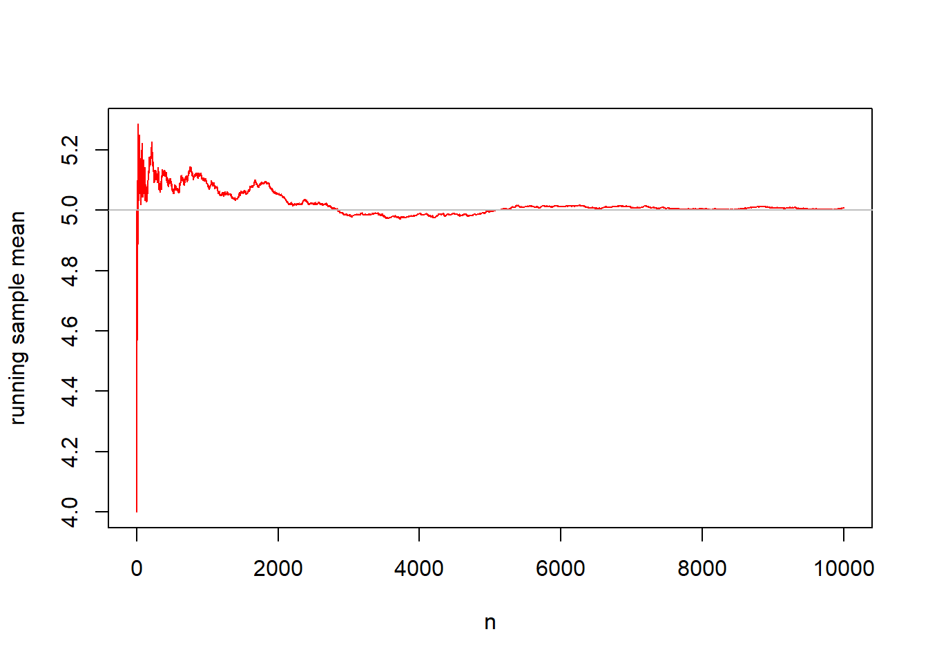
The second graph samples data from the Cauchy distribution \(f(x)=\frac{1}{\pi(1+x^2)}\) for \(-\infty < x < \infty\) and where \(\pi \approx 3.14\). This distribution is unusual in that it’s expected value is undefined. It has a median of zero. The running mean will appear to not converge for the Cauchy distribution.
##  [1]  0.3220090  2.9499724 -0.8523026 -0.1999247  5.3756972  0.8949486
## [7] -0.5757368 -2.5027118 3.4188212 -2.4518048## [1] 0.3220090 1.6359907 0.8065596 0.5549385 1.5190903 1.4150667 1.1306662
## [8] 0.6764939 0.9811969 0.6378968x.a <- 1:1000
plot(x.bar~x.a,ylab="running sample mean",xlab="n",
type="l",col="red")
abline(h=0,col="gray")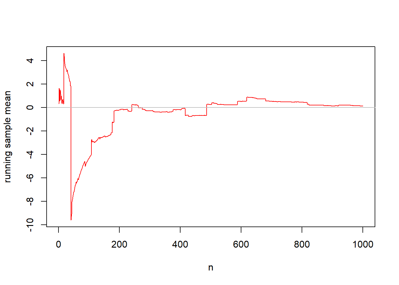
What if I look at running sample medians rather than means?
##  [1]   0.02949044  -8.32856849   0.25384241   6.53566865   1.87332442
## [6] 0.10692494 -14.07601384 -0.34631873 -0.00943959 1.00644251x.median<-1:1000
for (i in 1:1000) {
x.median[i]<-median(x[1:i])
}
x.median[1:10] #look at the first ten running medians## [1] 0.02949044 -4.14953903 0.02949044 0.14166642 0.25384241 0.18038367
## [7] 0.10692494 0.06820769 0.02949044 0.06820769x.a <- 1:1000
plot(x.median~x.a,ylab="running sample median",xlab="n",
type="l",col="red")
abline(h=0,col="gray")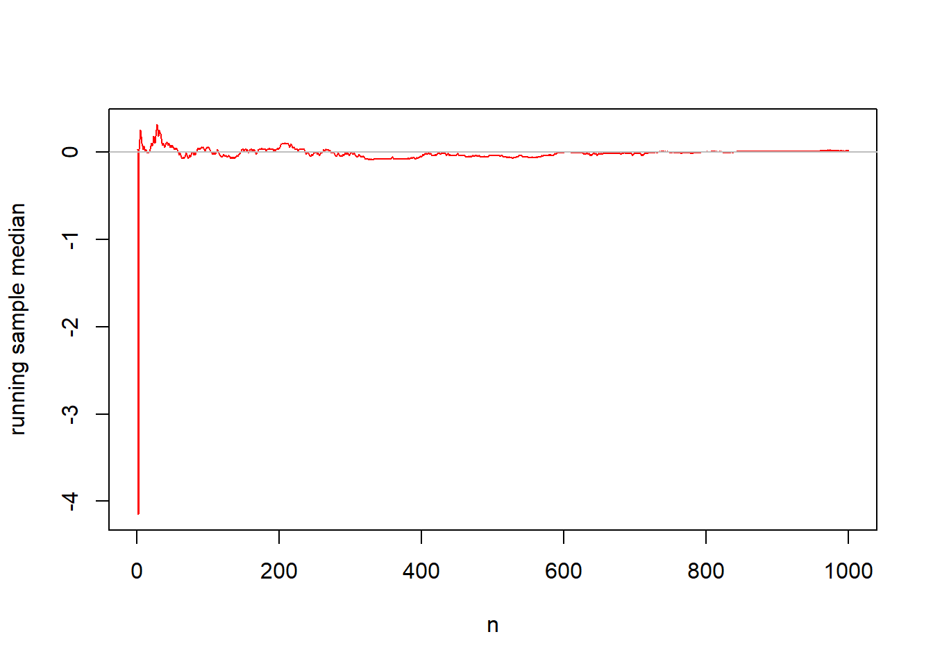
For the Cauchy distribution, the sample mean is NOT a consistent estimator of the population mean (because there is no population mean to converge to!), but the sample median is a consistent estimator of the population median. More about this at (http://www.johndcook.com/Cauchy_estimation.html).
Convergence in Distribution:
Let \(\{W_n\}=W_1,W_2,W_3,\cdots\) be an infinite sequence of random variables Let functions \(F_1,F_2,F_3,\cdots\) be the respective cdfs of \(\{W_n\}\) and functions \(M_1,M_2,M_3,\cdots\) be the respective mgfs of \(\{W_n\}\).
Lemma: If there is a random variable \(W\) and some interval containing zero such that for all \(t\) in that interval \[\lim_{n \to \infty} M_n(t)=M_W(t)\] then \[\lim_{n \to \infty} F_n(t)=F_W(t)\] for all \(w\).
We will not prove this lemma; basically it says that if the limit of a sequence of moment generating functions approaches the mgf of \(W\), then the limit of the cumulative distribution functions of the sequence will approach the cdf of \(W\).
Definition: The sequence of random variables \(\{X_n\}\) is said to converge in distribution (or law) to \(X\) if \[\lim_{n \to \infty} F_n(x) = F_X(x)\] (This also works with moment-generating function). When this happens, we write \[X_n \overset{D}{\rightarrow} X\] or \[X_n \overset{L}{\rightarrow} X\] Often we will say that \(X\) is the asymptotic distribution or the limiting distribution of \(X_n\).
A ‘stronger form’ of convergence is:
Definition: The sequence of random variables \(\{X_n\}\) is said to converge in probability to \(X\) if \[\lim_{n \to \infty} P(|X_n-X| \geq \epsilon)=0\] or equivalently \[\lim_{n \to \infty} P(|X_n-X| < \epsilon)=1\] When this happens, we write \[X_n \overset{P}{\rightarrow} X\]
It can be shown that \[X_n \overset{P}{\rightarrow} X \Longrightarrow X_n \overset{D}{\rightarrow} X\], but the converse is not true in general. If \(X=c\) (i.e. a constant, a so-called degenerate distribution), then convergence in distribution does imply convergence in probability.
Example: Let \(X_1,X_2,\cdots,X_n\) be an i.i.d. sample from \(X \sim UNIF(0,\theta)\) and we consider the maximum order statistic \(Y_n=max(X_1,X_2,\cdots,X_n)\). Intuitively, it seems like \(Y_n\) should ‘converge’ \(\theta\) as the sample size increases (i.e. if I take a large enough sample, my sample maximum eventually get \(\epsilon\)-close to \(\theta\)).
It can be shown (won’t prove here), that the cdf of the maximum order statistic is \[F_{Y_n}(x)=P(Y_n \leq x)=[F(x)]^n\]
Since \(f(x)=\frac{1}{\theta}\) for \(0 < x < \theta\) and hence \(F(x)=\frac{x}{\theta}\), then \(F_{Y_n}(x)=(\frac{x}{\theta})^n\) for \(0 < x < \theta\) (being equal to 0 when \(x \leq 0\) and 1 when \(x \geq \theta\)).
Now take the limit of the cdf of the sequence of random variables. The limit is zero when \(x < \theta\) and one when \(x \geq \theta\)–that’s a cdf of a degenerate distribution \(f(x)=1, x=\theta\). Hence \[Y_n \overset{D}{\rightarrow} \theta\] and because \(\theta\) is a constant \[Y_n \overset{P}{\rightarrow} \theta\]