Chapter 4 Bivariate Distributions

4.1 Bivariate Distributions of the Discrete Type

Definition of a joint probability mass function:

Given a random experiment with sample space $S$ and discrete random variables $X$ and $Y$, then the joint p.m.f. $f(x,y)$ is the function $f: \mathbb{R} \times \mathbb{R} \rightarrow \mathbb{R}$ that gives the probability that $X=x$ and $Y=y$ simultaneously, i.e. $f(x,y)=P(X=x \cap Y=y)$.

Example: Let $X$ represent the number of heads obtained when we flip a fair coin twice. The sample space is $S_X=\{0,1,2\}$. You should recognize that $X$ is binomial; $X \sim BIN(n=2,\pi=0.5)$.

Let $Y$ represent the result from rolling a standard six-sided die. Its sample space is $S_Y=\{1,2,3,4,5,6\}$. We often describe $Y$ as having a discrete uniform distribution with $n=6$.

In general, the p.m.f. for a discrete random variable $Y \sim DU(n)$ is: $$\begin{aligned} f(y) & = \frac{1}{n} \quad y=1,2,\cdots,n \\ & = 0 \quad otherwise \\ \end{aligned}$$

The sample space for the joint distribution of $X$ and $Y$ is all ordered pairs with non-zero probability. $$S=\{(0,1),(0,2),(0,3),\cdots,(2,4),(2,5),(2,6)\}$$

Eventually, we would like to have a formula to represent the joint pmf $f(x,y)$. First, we will consider the marginal distributions.

For $X$, we know that $$f(x)={2 \choose x}(0.5)^x (0.5)^{2-x}; x=0,1,2$$

Since $X$ is binomial, we can use the ‘shortcut’ formulas, rather than the definition, for finding the expected value and variance.

$$E(X)=n \pi=2 \times 0.5=1$$ $$Var(X)=n \pi (1-\pi)=\frac{1}{2}$$

Since $Y$ is discrete uniform, we have the following ‘shortcut’ formulas, which can be derived (exercise #64) using the defintions of expected value & variance, along with some of the summation formulas we found through proof by induction in Appendix B.

$$E(X)=\frac{n+1}{2}=\frac{7}{2}$$ $$Var(X)=\frac{n^2-1}{12}=\frac{35}{12}$$

Let’s look at a graph of the joint p.m.f. How do we get the probabilities that are shown?

JointPMF

Consider $f(1,1)$, the probability that both $X=1$ and $Y=1$. Since $X$ and $Y$ are independent, we can find $f(x,y)=f_X(x)f_Y(y)$. We would NOT be able to directly multiply if the variables were not independent.

$$f(1,1)=f_X(1) f_Y(1)=\frac{1}{2} \times \frac{1}{6}=\frac{1}{12}$$

Similarly, $f(0,2)$ and $f(2,6)$ are both equal to $\frac{1}{24}$.

$$f(0,2)=f_X(0) f_Y(2)=\frac{1}{4} \times \frac{1}{6}=\frac{1}{24}$$ $$f(2,6)=f_X(2) f_Y(6)=\frac{1}{4} \times \frac{1}{6}=\frac{1}{24}$$

So the joint pmf of $X$ and $Y$ is: $$\begin{aligned} f(x,y) & = \frac{1}{24} & x=0,2; y=1,2,3,4,5,6 \\ & = \frac{1}{12} & x=1; y=1,2,3,4,5,6 \\ \end{aligned}$$

or $$\begin{aligned} f(x,y) & = {2 \choose x}\frac{1}{24} x=0,1,2; y=1,2,3,4,5,6 \\ & = 0 otherwise \\ \end{aligned}$$

Now let’s look at a situation where we know the joint pmf and need to determine the marginal pmfs (i.e. the individual distributions of $X$ and $Y$). Also, we will determine if $X$ and $Y$ are independent or not.

Suppose the joint pmf for discrete random variables $X$ and $Y$ are:

$$f(x,y)=\frac{x+y}{32}, \quad x=1,2; y=1,2,3,4$$

(Draw a diagram to display $f(x,y)$, $f_X(x)$, $f_Y(y)$)

The marginal pmfs for $X$ and $Y$ are: $$\begin{aligned} f_X(x) & = \sum_y f(x,y) \\ & = \sum_{y=1}^4 \frac{x+y}{32} \\ & = \frac{x+1}{32}+\frac{x+2}{32}+\frac{x+3}{32}+\frac{x+4}{32} \\ & = \frac{4x+10}{32} \\ & = \frac{2x+5}{16} \quad x=1,2 \\ & = 0 \quad otherwise \\ \end{aligned}$$

4.2 The Correlation Coefficient

Recall that $Var(X+Y)=Var(X)+Var(Y)$ when $X$ and $Y$ are independent. What if they are NOT independent?

In that case, we have $$Var(X+Y)=Var(X)+Var(Y)+2E(XY)-2E(X)E(Y)$$ where the final two terms do NOT cancel out, due to the lack of independence. We define covariance as: $$Cov(X,Y)=E(XY)-E(X)E(Y)=E[(X-\mu_X)(Y-\mu_Y)]$$ .

Thus, the variance of the sum of two jointly distributed random variables is: $$Var(X+Y)=Var(X)+Var(Y)+2Cov(X,Y)$$

Obviously, if $X$ and $Y$ are independent, then $Cov(X,Y)=0$. However, the converse is not always true.

Let’s compute the covariance for our dependent discrete random variables $X$ and $Y$ where: $$f(x,y)=\frac{x+y}{32}, \quad x=1,2; y=1,2,3,4$$ $$f_X(x)=\frac{2x+5}{16}, \quad x=1,2$$ $$f_Y(y)=\frac{2y+3}{32}, \quad y=1,2,3,4$$

We need to compute $E(X)$, $E(Y)$, and $E(XY)$.

$E(X)=\frac{25}{16}, E(Y)=\frac{80}{32}=\frac{40}{16}$

$$\begin{aligned} E(XY) & =\sum_{x=1}^2 \sum_{y=1}^4 xy f(x,y) \\ & = (1)(1)\frac{1+1}{32} + (1)(2)\frac{1+2}{32} + \cdots + (2)(4)\frac{2+4}{32} \\ & = \frac{140}{32} \\ \end{aligned}$$

Hence $$Cov(X,Y)=\frac{140}{32}-\frac{25}{16} \times \frac{40}{16}=\frac{15}{32}$$ .

The covariance is hard to interpret. I have no idea if $Cov(X,Y)=\sigma_{XY}=\frac{15}{32}$ indicates a strong or weak degree of dependence between $X$ and $Y$. We typically ‘standardize’ covariance into a unitless version known as the correlation coefficient, denoted as $\rho$. The correlation coefficient has the property that $-1 \leq \rho \leq 1$.

$$\rho=\frac{Cov(X,Y)}{\sqrt{Var(X)\cdot Var(Y)}}=\frac{\sigma_{XY}}{\sigma_X \sigma_Y}$$ .

For our random variables, $$Var(X)=\frac{63}{256}, Var(Y)= \frac{45}{16}$$ .

So the correlation is $\rho=\frac{15/32}{\sqrt{63/256 \times 45/16 }}=\cdots=\frac{10\sqrt{35}}{105}=0.563$

Suppose we consider two independent random variables. Let $X \sim BIN(2,\frac{1}{2})$ and $Y \sim DU(4)$; that is, $X$ is the number of heads obtained by flipping 2 coins and $Y$ is the result of rolling a four-sided die.

For $X$, we have $E(X)=n \pi=2(\frac{1}{2})=1$ and $Var(X)=n \pi (1-\pi)=2(\frac{1}{2})(\frac{1}{2})=\frac{1}{2}$.

For $Y$, we have $E(Y)=\frac{n+1}{2}=\frac{5}{2}$ and $Var{Y}=\frac{n^2-1}{12}=\frac{15}{12}$

Since $$f(x)={2 \choose x}(\frac{1}{2})^x (\frac{1}{2})^{2-x}=\frac{1}{4}{2 \choose x}, \quad x=0,1,2$$ $$f(y)=\frac{1}{4}, \quad y=1,2,3,4$$ , then $$f(x,y)={2 \choose x}\frac{1}{16}, \quad x=0,1,2; y=1,2,3,4$$

The covariance term is: $$\begin{aligned} E(XY) & =\sum_{x=0}^2 \sum_{y=1}^4 xy f(x,y) \\ & = (0)(1){2 \choose 0}\frac{1}{16} + \cdots + (2)(4){2 \choose 2}\frac{1}{16} \\ & = \frac{40}{16}=\frac{5}{2} \\ Cov(X,Y) & = E(XY)-E(X)E(Y) \\ & = \frac{5}{2}-(1)(\frac{5}{2}) & = 0 \end{aligned}$$

Since Cov(X,Y)=0, then $\rho=0$.

Remember, when $X$ and $Y$ are independent, then $Cov(X,Y)=\rho=0$, but this lemma does not work in the other direction. That is, it is possible for $Cov(X,Y)=0$ when $X$ and $Y$ are not independent!

Example: Suppose that the joint pmf of $X$ and $Y$ is defined over three ordered pairs $(x,y)$ as follows: $$f(x,y)=\frac{1}{3}, \quad (x,y) \in \{(0,1),(1,0),(2,1)\}$$

If you draw the joint distribution, notice that the points do NOT form a Cartesian product or ‘rectangular’ support space. In this simple distribution, if I know that $Y=0$, then I am certain that $X=1$, hence they cannot be independent.

$f_X(x)=\frac{1}{3}, \quad x=0,1,2$ but $f_Y(y)=\frac{1}{3}, \quad y=0; f_Y(y)=\frac{2}{3}, \quad y=1$ and notice that $f(1,1)=0$ (the point (1,1) is not in our space) but that $f_X(1) \cdot f_Y(1)=\frac{1}{3} \times \frac{2}{3} \neq 0$, so $f(x,y) \neq f_X(x)\cdot f_Y(y)$ for at least some $(x,y)$. Thus, $X$ and $Y$ are not independent.

Let’s compute covariance. $$\begin{aligned} E(X) & = \sum x f(x) \\ & = 0(\frac{1}{3})+1(\frac{1}{3})+2(\frac{1}{3})=1 \\ E(Y) & = \sum y f(y) \\ & = 0(\frac{1}{3})+1(\frac{2}{3})=\frac{2}{3} \\ E(XY) & = \sum xy f(x,y) \\ & = 0(1)(\frac{1}{3})+(1)(0)(\frac{1}{3})+2(1)(\frac{1}{3}) = \frac{2}{3} \\ Cov(XY) & = E(XY)-E(X)E(Y) \\ & = \frac{2}{3}-1(\frac{2}{3})=0 \\ \end{aligned}$$

Thus, we have an example where two random variables are NOT independent but still have a covariance and a correlation of zero.

4.3 Conditional Distributions

We can find conditional distributions, where the conditional distribution is the ratio of the joint to the marginal.

$$\begin{aligned} f_{X|Y=y} & = \frac{f(x,y)}{f_Y(y)} \\ & = \frac{(x+y)/32}{(2y+3)/32} \\ & = \frac{x+y}{2y+3} \quad x=1,2; y=1,2,3,4 \\ \end{aligned}$$

For instance, $f_{X|y=1}=g(x|y=1)=\frac{x+1}{5}, x=1,2$/

Similarly, we can find the conditional distribution in the other direction.

$$\begin{aligned} f_{Y|X=x} & = \frac{f(x,y)}{f_X(x)} \\ & = \frac{(x+y)/32}{(4x+10)/32} \\ & = \frac{x+y}{4x+10} \quad x=1,2; y=1,2,3,4 \\ \end{aligned}$$

For instance, $f_{Y|x=2}=h(y|x=1)=\frac{2+y}{18}, y=1,2,3,4$/

We can find conditional means and variances just by applying the defintions of mean and variance.

$$\begin{aligned} E(X) & = \sum_x x f_X(x) \\ & = \sum_{x=1}^2 x \frac{4x+10}{32} \\ & = 1 \times \frac{14}{32} + 2 \times \frac{18}{32} \\ & = \frac{50}{32} = 1.5625 \end{aligned}$$ $$\begin{aligned} E(X|y=1) & = \sum_x x g(x|y=1)) \\ & = \sum_{x=1}^2 x \frac{x+1}{5} \\ & = 1 \times \frac{2}{5} + 2 \times \frac{3}{5} \\ & = \frac{8}{5} = 1.6 \end{aligned}$$

Notice that $E(X) \neq E(X|y=1)$.

$$\begin{aligned} Var(X) & = E(X^2)-[E(X)]^2 \\ & = \sum_x x^2 f_X(x)-(\frac{50}{32})^2 \\ & = \sum_{x=1}^2 x^2 \frac{4x+10}{32} - (\frac{25}{16})^2 \\ & = 1^2 \times \frac{14}{32} + 2^2 \times \frac{18}{32}-\frac{625}{256} \\ & = \frac{63}{256} = 0.2460938 \end{aligned}$$

$$\begin{aligned} Var(X|y=1) & = E(X^2|y=1)-[E(X|y=1)]^2 \\ & = \sum_x x^2 g(x|y=1)-(\frac{8}{5})^2 \\ & = \sum_{x=1}^2 x^2 \frac{x+1}{5} - (\frac{8}{5})^2 \\ & = 1^2 \times \frac{2}{5} + 2^2 \times \frac{3}{5}-\frac{64}{25} \\ & = \frac{6}{25} = 0.24 \end{aligned}$$ Again, $Var(X) \neq Var(X|y=1)$.

Are the random variables $X$ and $Y$ independent? If they are, then the joint pmf is equal to the product of the marginal pmfs (i.e. the joint pmf can be factored into the pmfs for the two individual random variables)?

We have $f(x,y)=\frac{x+y}{32}$, $f_X(x)=\frac{2x+5}{16}$, and $f_Y(y)=\frac{2y+3}{32}$.

Clearly $X$ and $Y$ are not independent, as $$\frac{2x+5}{16} \times \frac{2y+3}{16} \neq \frac{x+y}{32}$$

4.4 Bivariate Distributions of the Continuous Type

A joint probability density function (pdf) is some function $f: \mathbb{R}^k \to \mathbb{R}$ such that:

• $f(x_1,x_2,\cdots,f_k)=f($ x $)\geq 0$ for all x $\in \mathbb{R}^k$

• $\int_{-\infty}^\infty \int_{-\infty}^\infty \cdots \int_{-\infty}^\infty f(x_1,x_2,\cdots,x_n) dx_1 dx_2 \cdots dx_n = \int_{x \in \mathbb{R}^k} f($ x $) d$ x $=1$

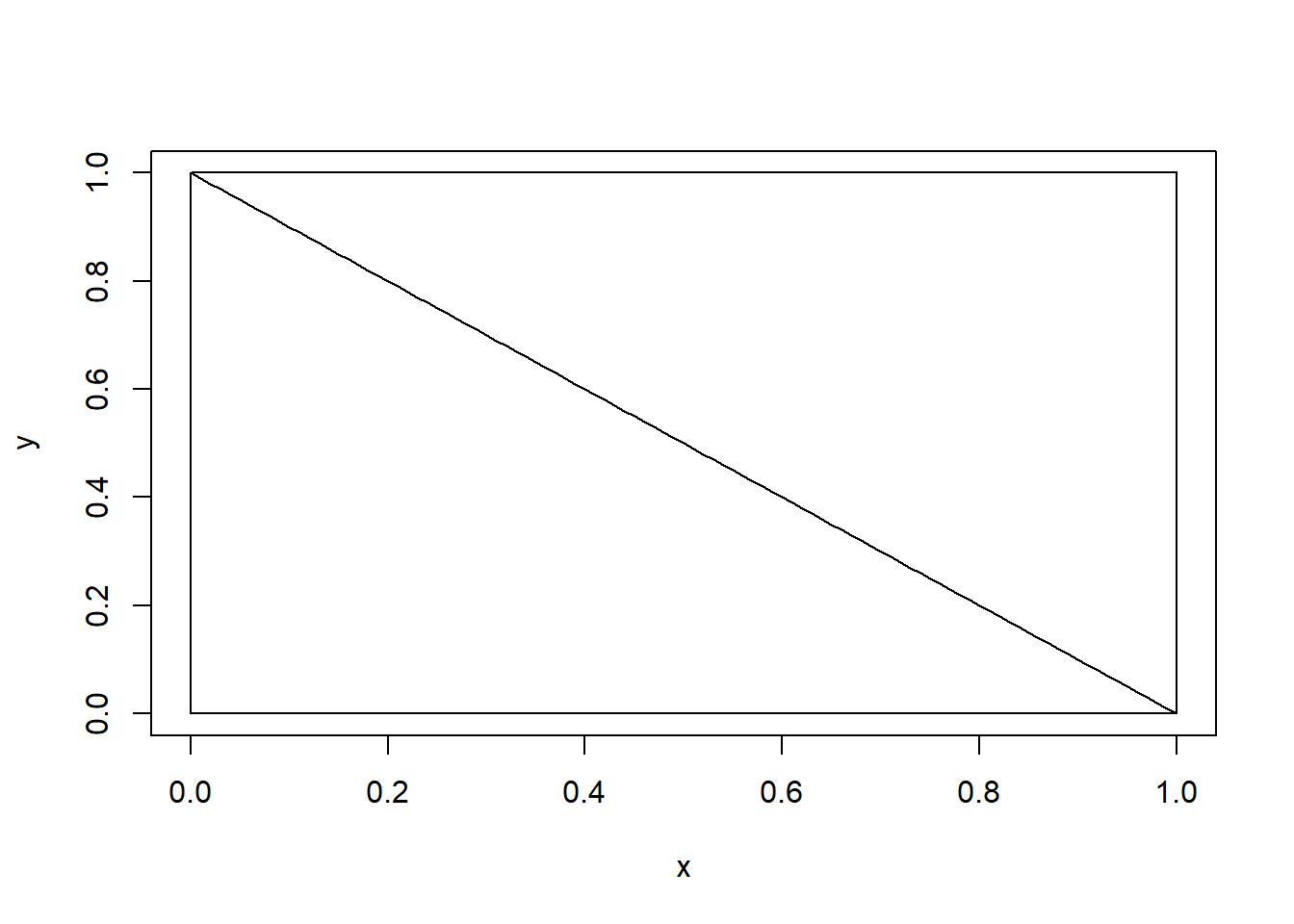
Example: Let $X$ and $Y$ have joint pdf $$f(x,y)=x+y, 0 < x < 1, 0 < y < 1$$

The marginal pdfs are easily obtained by integrating out the other variable.

$$f_X(x)= \int_0^1 x+y dy = xy+\frac{y^2}{2}|_0^1 = x+\frac{1}{2}, 0 < x <1$$

Similarly, $f_Y(y)=y+\frac{1}{2}, 0 < y <1$

Suppose I want the probability $P(X+Y \leq 1)$. I must use the joint pdf to evaluate this.

$$\begin{aligned} P (X+Y \leq 1) & = \int_0^1 \int_0^{1-x} (x+y) dx dy \\ & = \int_0^1 [xy+\frac{y^2}{2}]_0^{1-x} dx \\ & = \int_0^1 x(1-x)+\frac{(1-x)^2}{2} dx \\ & = \int_0^1 x-x^2+\frac{1}{2}-x+\frac{1}{2}x^2 dx \\ & = \int_0^1 \frac{1}{2}-\frac{1}{2}x^2 dx \\ & = \frac{x}{2}-\frac{x^3}{6}|_0^1 \\ & = \frac{1}{2}-\frac{1}{6} \\ & = \frac{1}{3} \end{aligned}$$

Geometrically, this probability is the volume under the surface $f(x,y)=x+y$ above the set $\{(x,y): 0 < x,x+y \leq 1 \}$.

The conditional distribution is defined similarly as before, with Conditional = $\frac{Joint}{Marginal}$

$$g(x|y)=f_{X|Y=y}=\frac{f(x,y)}{f_X(x)}$$ In our example, $g(x|y)=\frac{x+y}{x+1/2}, 0 < x < 1$.

Another example of a joint pdf

Suppose that $f(x,y)=\frac{1}{40}, 0 \leq x \leq 10, 10-x \leq y \leq 14-x$

Do the following:

1. Draw the support space $\mathcal{S}_{XY}$.

2. Find the marginal pdf for $X$, $f_X(x)$

3. Find the conditional pdf for $Y|X=x$, $f_{Y|X=x}(y)$ or $g(y|x)$

4. Find the conditional expectation $E(Y|x)$

5. Find the conditional variance $Var(Y|x)$

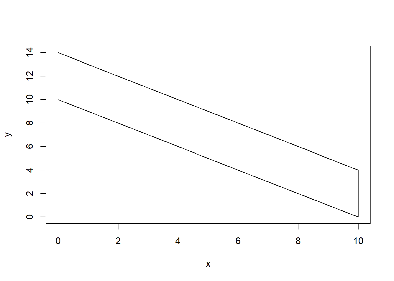
Notice that $X$ and $Y$ are not independent. The support space $\mathcal{S}_{XY}$ is not rectangular with the support of $Y$ depends upon the value of $X$.

Find the marginal pdf for $X$.

$$\begin{aligned} f_X(x) = & \int f(x,y) dy \\ = & \int_{10-x}^{14-x} \frac{1}{40} dy \\ = & \frac{y}{40}|_{10-x}^{14-x} \\ = & \frac{14-x}{40}-\frac{10-x}{40} \\ = & \frac{4}{40}=\frac{1}{10}, 0 \leq x \leq 10 \\ \end{aligned}$$ Notice that $X \sim UNIF(0,10)$.

Find the conditional pdf for $Y$ given $X$.

$$\begin{aligned} g(y|x) = & \frac{f(x,y)}{f_X(x)} \\ = & \frac{1/40}{1/10} \\ = & \frac{1}{4}, 10-x \leq y \leq 14-x, 0 \leq x \leq 10 \\ \end{aligned}$$

Notice that $Y \sim UNIF(10-x,14-x)$.

The conditional expectation is:

$$\begin{aligned} E(Y|x) = & \int y g(y|x) dy \\ = & \int_{10-x}^{14-x} \frac{y}{4} dy \\ = & \frac{y^2}{8}|_{10-x}^{14-x} \\ = & \frac{(14-x)^2}{8}-\frac{(10-x)^2}{8} \\ = & \frac{(196-28x+x^2)-(100-20x+x^2)}{8} \\ = & \frac{96-8x}{8} \\ = & 12-x \\ \end{aligned}$$ So if $X=5$, then $E(Y|X=5)=12-5=7$.

The conditional variance is:

$$\begin{aligned} E(Y^2|x) = & \int y^2 g(y|x) dy \\ = & \int_{10-x}^{14-x} \frac{y^2}{4} dy \\ = & \frac{y^3}{12}_{10-x}^{14-x} \\ = & \frac{(14-x)^3}{12}-\frac{(10-x)^3}{12} \\ \end{aligned}$$

Recall that $(x-y)^3=x^3-3x^2y+3xy^2-y^3$, so

$$\begin{aligned} E(Y^2|x) = & \frac{(2744-588x+42x^2-x^3)-(1000-300x+30x^2-x^3)}{12} \\ = & \frac{1744-288x+12x^2}{12} \\ = & \frac{436}{3}-24x+x^2 \\ Var(Y|x) = & E(Y^2|x)-[E(Y|x)]^2 \\ = & (\frac{436}{3}-24x+x^2)-(12-x)^2 \\ = & (\frac{436}{3}-24x+x^2)-(144-24x+x^2) \\ = & \frac{436}{3}-144=\frac{4}{3} \\ \end{aligned}$$

If I had defined $X \sim UNIF(0,10)$ and $Y \sim UNIF(0,4)$ such that $X$ and $Y$ were independent, then $$f(x,y)=f_X(x) \times f_Y(y) = \frac{1}{10} \times \frac{1}{4} = \frac{1}{40}, 0 \leq x \leq 10, 0 \leq y \leq 4$$

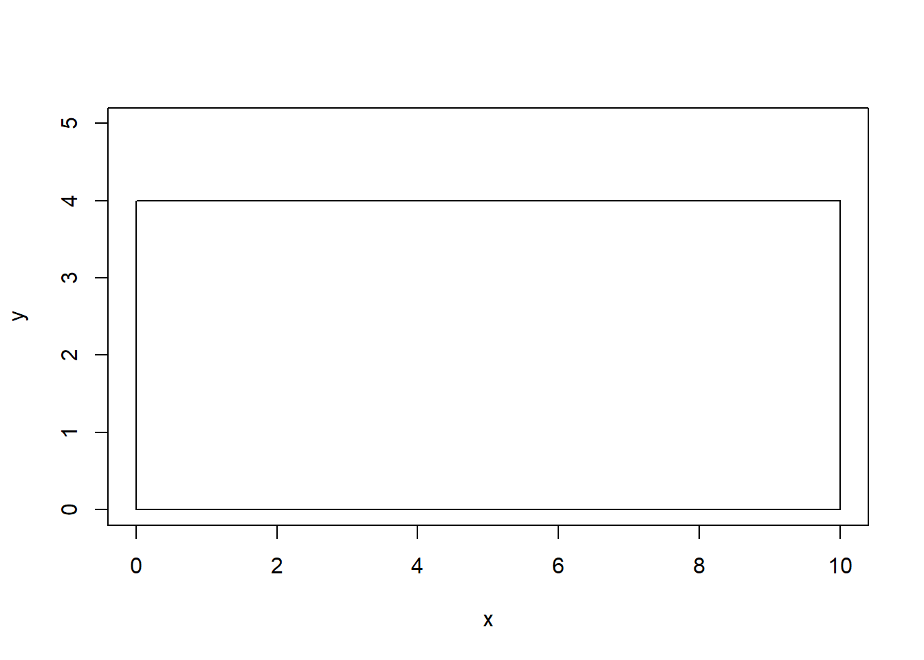
Of course, the support space in now rectangular (although that does NOT guarantee independence) and the support for $Y$ no longer depends on $X$.

4.5 The Bivariate Normal Distribution